Intersect Operator in Excel offers a powerful way to analyze data by identifying the intersection of two or more ranges. By using this operator, you can pinpoint the exact cells where data overlaps, providing valuable insights into relationships and correlations within your dataset. Say goodbye to complex formulas and hello to a more intuitive method of data analysis. Whether you’re comparing sales figures, tracking inventory levels, or conducting demographic analysis, the Intersect Operator in Excel streamlines your workflow and enhances your ability to extract meaningful insights from your data. Embrace this versatile tool to unlock new possibilities for data exploration and decision-making. With the Intersect Operator, you can effortlessly identify intersections and uncover hidden patterns in your Excel spreadsheets, empowering you to make informed choices and drive success in your projects.
This Tutorial Covers:
- Intersect Operator in Excel
- Intersection of a Single Row and Column
- Intersection of a Multiple Rows and Columns
- Intersection of Named Ranges
- A Real-World Excel Intersect Operator Example
1. Intersect Operator in Excel
The intersect operator in Excel is used to determine where two ranges meet. It is represented by the space character (“”).
The region where two ranges overlap or collide is referred to as the intersection of two ranges.
Excel Intersect Function can be used to determine:
- The intersection of a single row and column.
- The intersection of multiple rows and columns.
- The intersection of Named Ranges.
2. Intersection of a Single Row and Column
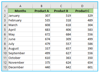
Consider the data collection depicted below:
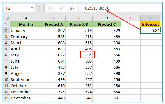
If you use =C2:C13 B6:D6 right now The intersect operator in Excel will yield 684 (the value in column C6), which represents the intersection of these two ranges [note that there is only one space between the ranges].
3. Intersection of a Multiple Rows and Columns
The intersection in Excel of ranges that cover more than one row or column can be found using the same method. You can obtain the intersection of Products 1 and 2 in June using the same data collection as above.
The equation for doing that is as follows:
=B2:C13 B7:D7
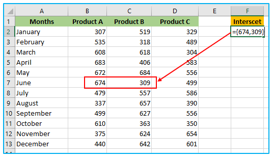
When you select the formula and press F9, the result will appear as “={674,309,}” despite the fact that the formula’s result would normally indicate a Value error. The intersection numbers are returned as an array by this formula. This can be incorporated into formulas like SUM or MAX to determine the intersection numbers’ sum (to get the maximum of the intersection values).
4. Intersection of Named Ranges
Using Excel’s Intersect Operator, you can also locate the intersection using named ranged cells intersection.
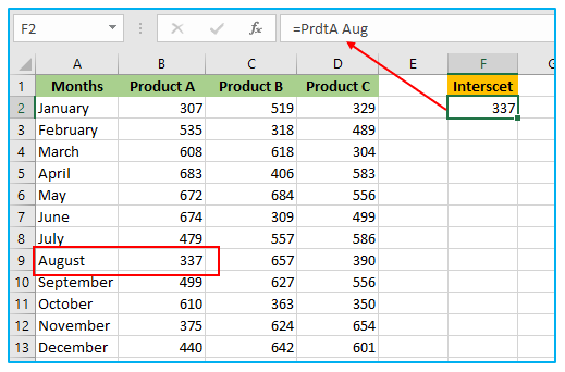
Here is an illustration where I have labeled the numbers for Product A and B as PrdtA and PrdtB, month August as Aug.
Now you can use the formula =PrdtA Aug to determine where these two ranges meet.
5. A Real-World Excel Intersect Operator Example
This is an instance where the technique might be useful. I have statistics on each employee’s monthly sales for 2022.
In order to extract the sales that the Employee made during that month, I have also constructed a drop-down list with the Employee Name and Month Name in separate cells.
How to accomplish this:
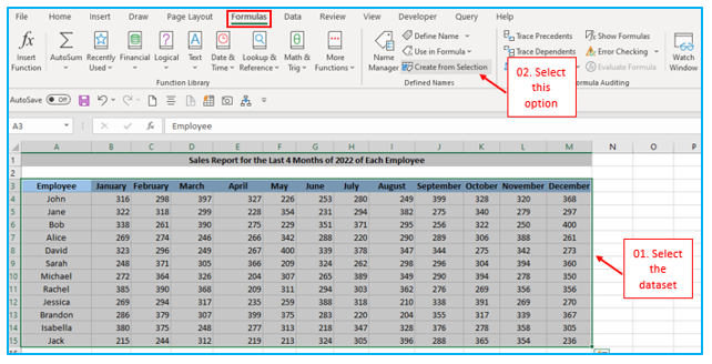
Step 1: To create named ranges, select the full data set (A3:M15) and press Control + Shift + F3. (Alternatively, you can do it by selecting Formula -> Defined Names -> Create from Selection.) A dialogue window labeled “Create Names from Selection” will then appear.
Step 2: Click OK after choosing “Top Row” and “Left Column.”
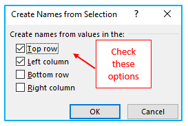
By doing this, named groups will be created for every Employee Name and every Month.
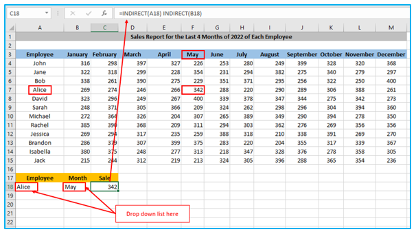
Step 3: Create a drop-down list for each Employee Name in column A18 now. Likewise, go to cell B18 and set up a drop-down menu for each month. Use the following formula in cell C18: =INDIRECT(A18) INDIRECT(B18)
How does it work?
There is a blank area between the two INDIRECT formulas, as you can see.
The space between them acts as an intersect operator and returns the intersecting value. The INDIRECT function returns the range for the specified ranges, Employee, and the Month.
Application of Intersect Operator in Excel
- Data Analysis: Utilize the Intersect Operator in Excel to identify common data points between multiple datasets, facilitating comprehensive data analysis and comparison.
- Conditional Formatting: Apply conditional formatting rules using the Intersect Operator to highlight cells where specific conditions are met at the intersection of two or more ranges.
- Venn Diagram Creation: Create Venn diagrams in Excel by using the Intersect Operator to determine the overlapping areas between different sets of data, aiding in visual representation and analysis.
- Data Validation: Implement data validation rules that depend on the intersection of two or more ranges, ensuring data integrity and consistency across your Excel worksheets.
- Dynamic Named Ranges: Define dynamic named ranges using the Intersect Operator to refer to cells that intersect between multiple ranges, allowing for flexible and efficient data referencing.
- Error Checking: Use the Intersect Operator to detect errors or inconsistencies by identifying cells that intersect between a reference range and a validation range, facilitating data validation and quality assurance processes.
For ready-to-use Dashboard Templates:
