How to use the Quotient function in Excel

QUOTIENT function in Excel returns only the integer part of the result and discards the remainder. It can be very handy for division, but only useful for the whole number of its resulting integers. The quotient can be used to find the result of integer division by specifying the dividend and the divisor in the input.

What is Excel Quotient Function?
Apply Cell Reference for Quotient in Excel.
Apply QUOTIENT Function to return integer portion.
Using Division operator (/) and Quotient function
Apply Direct Numeric Values for Quotient in Excel.

What is Quotient function in Excel?

In Excel, the quotient function is a mathematical expression that can be used to determine the integer result of dividing. This method essentially involves diluting integers and neglecting the remainder. This is useful when the result of a division is only an integer and you want to discard all decimal parts.

Syntax of Quotient Function =QUOTIENT(numerator, denominator)

numerator: The dividend, or the number to be divided.

denominator: The divisor, or the number by which the numerator is to be divided.

How to use Cell Reference for Quotient in Excel?

There are steps for use of Quotient function. The steps are below: –

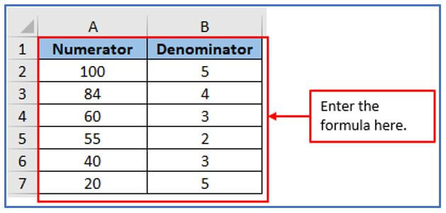
Step 1: Pick some numbers and Denominator and create a data table with the data’ as shown below.

Written the name here.

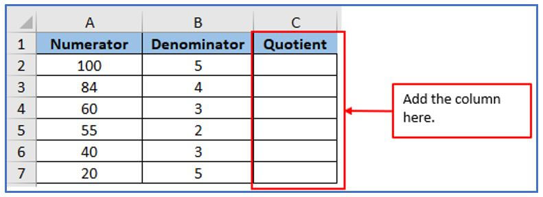
Step 2: Add the columns from C1:C7 to get the Quotient output there.

Added the column here.

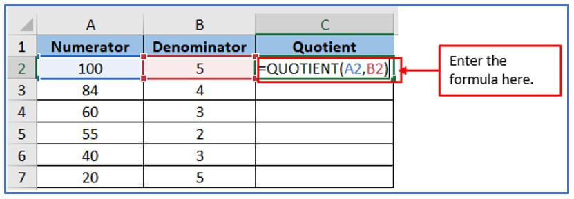
Step 3: You can refer to the Quotient function and refer to C2 for enter the formula.

The formula is: =QUOTIENT(A2,B2)

Using the columns A2 and B2, which respectively translate to A2/B2.

Used the formula here.

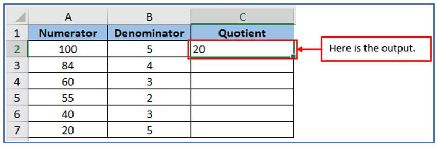
Step 4: In the end, hit enter to get the Quotient output.

Here is the result below.

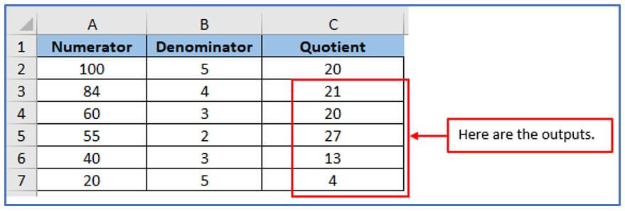
Step 5: Use the same formula here or drag-down the cursor from C2:C7 to get the rest of the outputs.

Here are all the Quotient outputs.

Apply QUOTIENT Function to return integer portion.

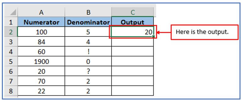
Step 1: Make a table with some integer values and some special characters.

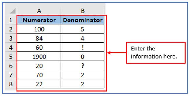
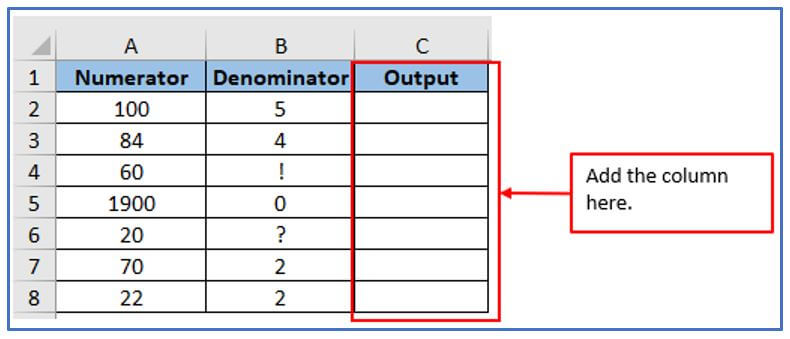
Step 2: Add another column C1:C8 to get the QUOTIENT Function output there.

You can see below the column has been added here.

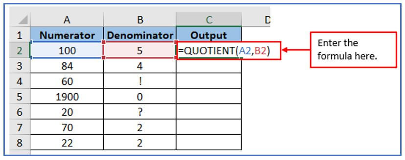
Step 3: Enter the formula now. The formula: =QUOTIENT(A2,B2)

Applied the formula here.

Step 4: After entering the formula press enter button.

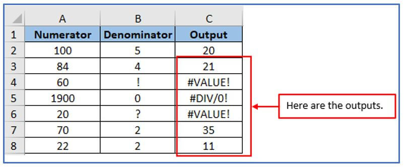
Here is the result is shown below.

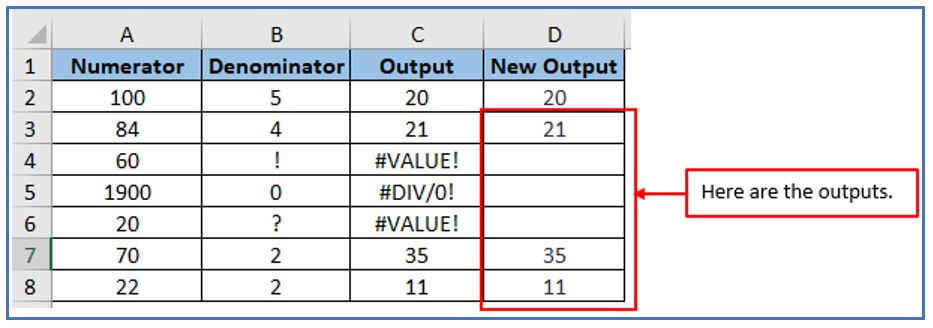
Step 5: You can see this #VALUE! in cell C4 because of the special characters. #DIV/0! error in column C5. This is because the QUOTIENT function returns a DIV error if the specified argument is not an integer value the denominator is zero (0). C6 This contains special characters that cause the QUOTIENT function to return a VALUE error in the result below.

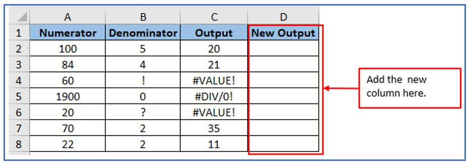
Step 6: Add another column D1:D8 to get rid of the above problem.

Step 7: To solve the issue, I implemented an ISERROR function with an optional argument that checks for error (#N/A, #VALUE. #DIV/0, “NUM”) and returns either TRUE or FALSE. The formula uses QUOTIENT within ISERROR. The formula: =IF(ISERROR(QUOTIENT(A2,B2)),””,QUOTIENT(A2,B2))

Applied the formula here.

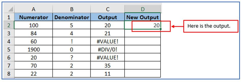
Step 8: After entering the new formula press enter.

Here is the result.

Step 9: Then drag the formula from D2 to D8 to all cells to get the following output: In the following results, you can see that the DIV and VALUE errors did not occur after applying the formula.

This returns empty output because we use double quotes after the QUOTIENT function to check for errors and return empty output if any are found. So, you will get an empty output for each error.

Using Division operator (/) and Quotient function.

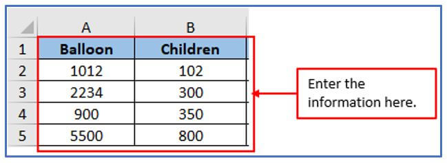
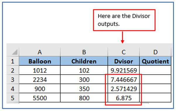
Step 1: Observe the following statement concerning a group of Balloons and children. The number of Balloons each child will receive is what you need to figure out. Utilize both the division operator and QUOTIENT function in Excel to obtain precise results, as demonstrated below.

Step 2: Add the columns from C1:C5 for getting the output of Divisor and add the columns from D1:D5 for getting the Quotient result.

The Column is added here.

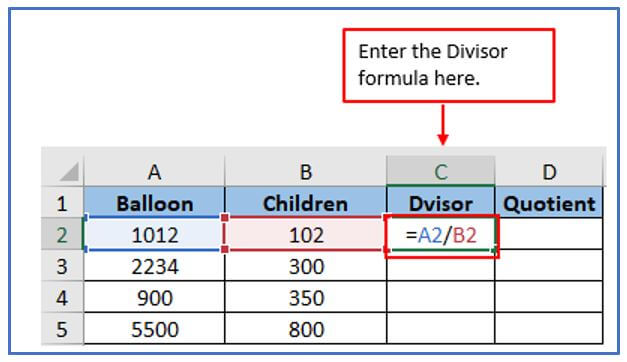
Step 3: Here you can refer to the Divisor formula in cell C2 to get the output. The formula: =A2/B2

Step 4: Click on the Enter button to get the result.

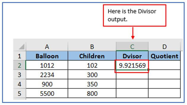
The Divisor result is outlined below.

Step 5: To get the rest of the Divisor outputs use the same formula for cell C3: or drag-down the formula from C2:C5.

In the given result, it is evident that a decimal was used to compute the division operator. This is because the slash (/) and the division symbol return a decimal number with a larger value if there is a remainder after the division number. Confusion arises as to exactly how much balloons to give each child.

Step 6: To solve the above confusion, use the Quotient formula. The formula: =QUOTIENT(A2,B2)

Step 7: Press the enter tab.

Here is the Quotient result:

Step 8: It is now possible to determine how many balloons are given to each child. Use the same formula or drag-down the cursor from D2:D5. Consider the first number containing 1012 balloons and 102 children. Therefore, out of 102 children, each child will receive 9 pieces of balloons.

Here are all the Quotient outputs.