How to use the moving average formula in Excel?

Average formula in Excel is a fundamental tool for calculating the mean of a range of values. By using the average formula in Excel, you can quickly summarize data, identify trends, and analyze performance across various datasets. Whether you’re working with financial reports, sales data, or statistical information, this formula helps streamline calculations and improve accuracy. Incorporating the average formula in Excel into your workflow will not only save time but also enhance your ability to make data-driven decisions with ease. Optimize your data analysis by mastering the average formula in Excel.

What is the moving average?
How to calculate simple moving averages in Excel?
How to calculate the moving average for the last N days (weeks, months, years)?
How to calculate the moving average for the last N values in a row?
Some tips for using moving average formula in Excel

1. What is moving average?

By using a moving average, market analysts and investors can identify the direction of underlying trends. It summarizes a financial security’s data points over a specific period and takes the average by dividing the sum by the number of data points. It is called a “moving” average because it is continuously recalculated based on the latest price data. Analysts use moving averages to evaluate the movement of an asset’s price to find support and resistance. Moving averages reflect the previous price movement/movement of a security. Analysts and investors then use that information to determine the potential direction of the asset’s price.

They are called lagging indicators because they generate signals according to the price movements of the underlying asset or indicate the direction of a particular trend.

Investors and traders use a moving average to gauge the direction of underlying security trends.
Multiply the number of periods by the addition of all the data points within a specific period.
The use of moving averages enables technical traders to generate trading signals.

2. How to calculate simple moving averages in Excel?

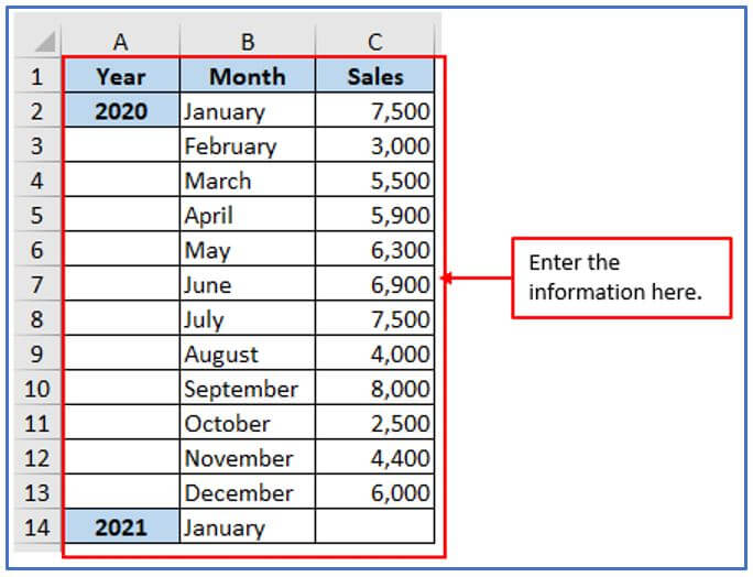
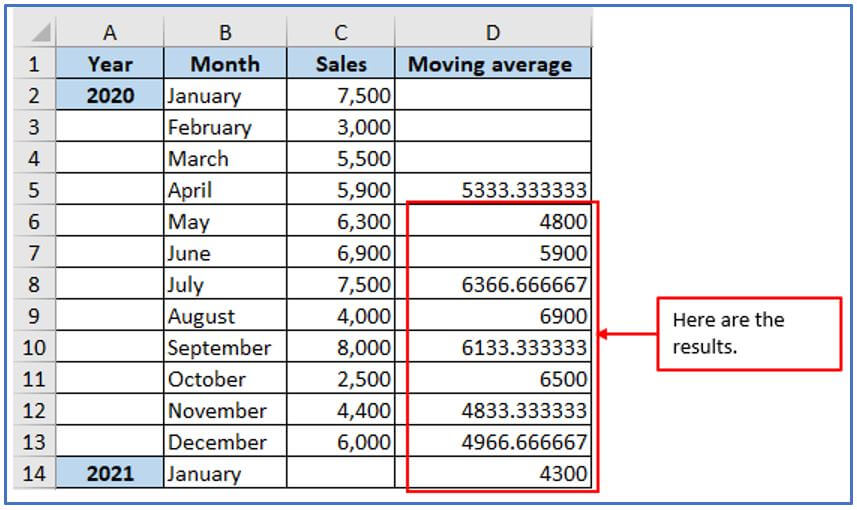
The simple moving average was calculated using sales data from companies during the January to December 2020 period. The objective is to find out the sales data and determine the comparable sales for January here. For this reason, here used 3 months of sales to determine the moving average for January, February, and March, then divide sales by 3 for each month.

Step 1: Create a table with the above information.

Create the table here.

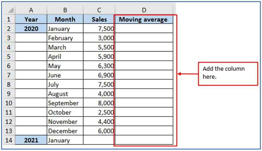
Step 2: Add the column from D1:D14 to get the result there.

Add the column here.

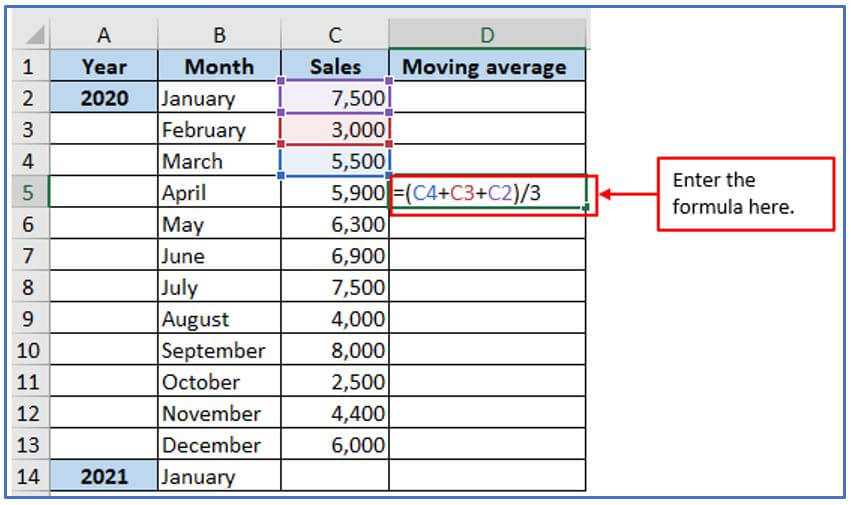
Step 3: Here is simple moving averages formula. The formula will be applied in cell D5 because here wanted to find the simple moving average of January month and as we know for this you need to plus three months’ sales and divided by three that’s why.

The formula is: =(C4+C3+C2)/3

Apply the formula here you can see below.

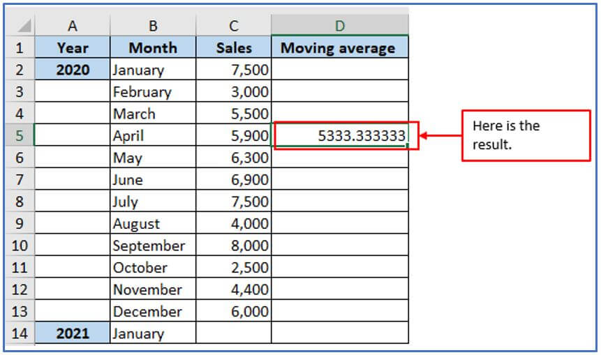
Step 4: In the end, hit enter to get the today’s date.

Here is the January month simple moving average result below.

Step 5: Now, drag-down the cursor from D5:D14.

Here Sales are expected to be at 4,300 by January.

3. How to calculate the moving average for the last N days (weeks, months, years)?

Here you have the sales for January- December. You want to know the average for the last 3 months (September, October, and November). To do this, you need a formula that recalculates the average. Here enter an average value with offset and count in the past.

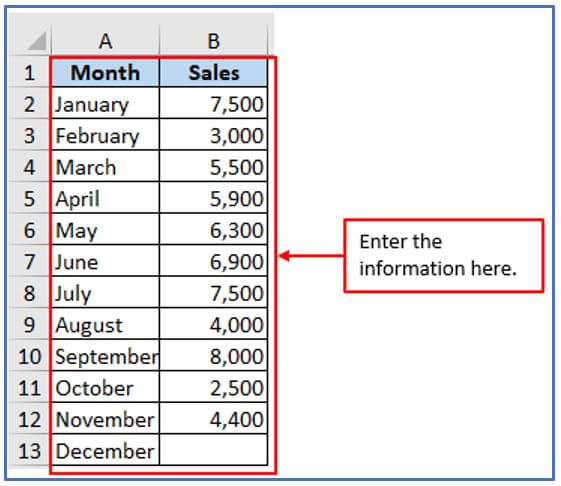
Step 1: Make a table first with Month and Sales.

Form the column here.

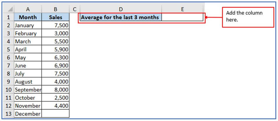
Step 2: Add a column in D1 and E1 to get the last 3 months simple moving average value.

The column has been added here.

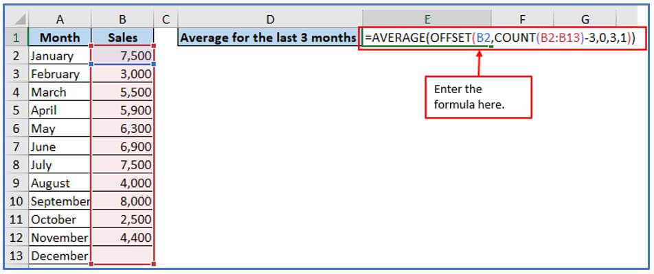
Step 3: You just need to refer to the in-cell E1. The formula is:

=AVERAGE(OFFSET(first cell, COUNT(entire range)N,0,N,1))

=AVERAGE(OFFSET(B2,COUNT(B2:B19)-3,0,3,1))

Where N is the number of past days/weeks/months/years included in the average.

The count of values that have been entered in column B by the function COUNT(B2: B19) is a count.So, start counting from B2 because it is the header.

The OFFSET function uses cell B2 (first argument) as the starting point and moves the count (the value returned by the COUNT function) up three rows (-3 in the second argument). The result is the sum of the values in a range of 3 rows (3 in the fourth argument) and 1 column (1 in the last argument), that is, the required last three months.

Place the formula here.

Step 4: Now press enter to get the average for the last 3 months (September, October and November).

Here is the Now value below.

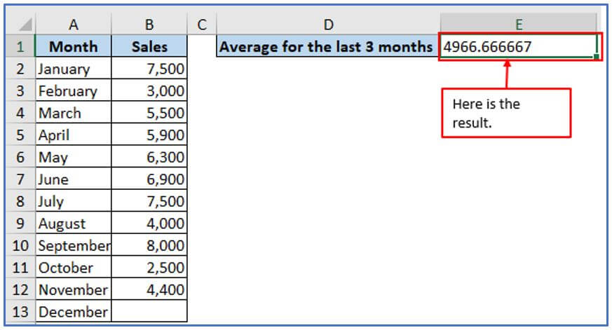
4. How to calculate the moving average for the last N values in a row?

Here you have the sales for January- December. You want to know the average for the last 3 months (September, October and November). To do this, you need a formula that recalculates the average. Here enter an average value with offset and count in the past.

Step 1: Enter the information into your excel as shown below.

Write down the dates into the Excel sheet here.

Step 2: Add a column in A4 and B4 to get the output.

Added the column here.

Step 3: You just need to refer to the in-cell E1. The formula is:

=AVERAGE(OFFSET(first cell, COUNT(entire range)N,0,N,1))

=AVERAGE(OFFSET(B2,0,COUNT(B2:M2)-3,1,3))

Where N is the number of past days/weeks/months/years included in the average.

The count of values that have been entered in column B by the function COUNT(B2:M2) is a count. The OFFSET function uses cell B2 (first argument) as the starting point and moves the count (the value returned by the COUNT function) up three rows (-3 in the second argument). The result is the sum of the values in a range of 3 rows (3 in the fourth argument) and 1 column (1 in the last argument), that is, the required last three months.

Used the formula here.

Step 4: Now press enter to get the average for the last 3 months (September, October and November).

Here is the Now value below.

5. Some tips for using the moving average formula in Excel.

Here are a few Excel moving average formula tips.

Select appropriate window size: Depending on the size of the window, each average calculation includes a certain number. Reducing the window size makes it more responsive to changes, but can be noisier. However, if you increase the size of your window, it will smooth out the average but may cause delays.
Consider the frequency of the data: In case your data consists of daily, weekly, or monthly observations. Determine the window size that corresponds to the frequency of your data usage. It is possible to use a 7-day moving average for daily data and retrace it with ten months’ worth of monthly data.
Use absolute references: When copying formulas, especially when dragging formulas across multiple cells, always use absolute references at the start and end of the range. This prevents the area from shifting when the formula is copied.
Handling missing or incomplete data: Determine how to handle missing or incomplete data points. Depending on your data and analysis needs, you can ignore them, replace them with zero, or use other interpolation methods.
Visualizing moving averages: After calculating moving averages, you should consider creating graphs to visualize trends over time. Plotting both the original data and the moving average provides insight into patterns and trends.
Experiment with different types of moving averages: Although the default moving average for Excel, AVERAGE, can also be used to calculate other types of moving Averages, such as weighted or exponential moving averages. You can also look at the moving average.
Using Named Ranges: If you have large data sets or want to make your formulas more readable, consider using named ranges to reference the data range for moving average calculations.
Test and validate the results: To make a final determination before using an average, either run the calculations manually or check for accuracy.

These tips can help you use Excel’s moving average formula to analyze trends and patterns in your data while avoiding common mistakes.

Application of Average Formula in Excel

Financial Analysis: Use the average formula in Excel to calculate the mean of financial data, such as expenses or revenue, for performance evaluation.
Performance Tracking: Track employee performance or sales metrics by averaging key indicators over time for consistent analysis.
Sales Forecasting: Average past sales figures to forecast future trends and make informed business decisions.
Grade Calculation: Calculate students’ average grades from multiple tests or assignments, making academic evaluations easier.
Inventory Management: Determine average stock levels or consumption rates to optimize inventory control and reduce waste.
Data Trend Analysis: Use averages to smooth out fluctuations in large datasets, identifying overall trends and patterns in your data.