Excel SCAN Function, a term used in Excel, is the systematic exploration or analysis of data to identify specific patterns, values, or characteristics within. Although Excel does not have a special feature called a “scan feature,” you can use a variety of built-in features and functions for scanning tasks.
Topics covered:
- Syntax of scanning function in Excel
- How to use the scanning function Cumulative Summation in Excel?
- How to use the scanning function Cumulative Average in Excel?
- How to use the scanning function Cumulative Max in Excel?
- Tips for scanning function in Excel.
1.Syntax of scanning function in Excel
=SCAN ([initial_value], array, lambda(accumulator, value, body))
The SCAN function syntax has the following arguments and parameters:
[initial_value] Obtains the commencement value of the accumulater.
Array to scan.
LAMBDA called to collapse a Lambda array. LAMBDA requires three parameters.
Accumulator the sum value is returned as the final result.
Value Current value from the array.
Body every element within the array undergoes a calculation.
2. How to use the scanning function Cumulative Summation in Excel?
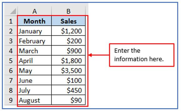
Step 1: First create a dataset with the names of the months and the sales like the image below.
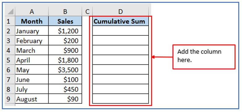
Step 2: Add the column in A1:A5 to get the Cumulative Summation there.
A column has been added you can see it below.
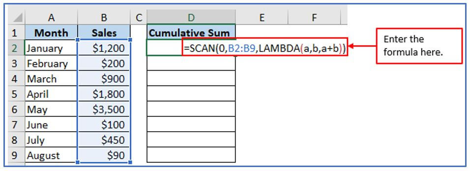
Step 3: Two parameters and an expression are combined to form the LAMBDA function of the SCAN function. Cumulative sums are always cumulative, meaning that the accumulator adds values on each iteration, but this does not necessarily mean that all cases are equal. The output of the previous LAMBDA function from the preceding element is what we call the accumulator in practical terms.
Now, type this formula: =SCAN(0,B2:B9,LAMBDA(a,b,a+b))
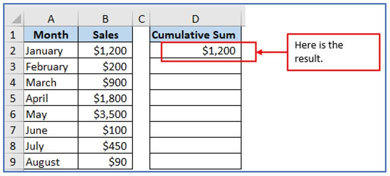
Step 4: After entering the formula press enter. The accumulation (a) starts from the beginning. Value (b) starts from the first cell in the range. It calculates the sum of both as there is no “a” here, that’s why the result is the same as B2.
Here is the output.
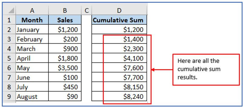
Step 5: It calculates the sum of both. The LAMBDA function’s output is represented by the accumulator (a). The current element of an array can be represented by the value parameter (b)It’s time to copy this formula into the remaining cells of the column. Just double-click or hold the fill handle and drag it down (located at the bottom right of cell here D2).
Here are all the results.
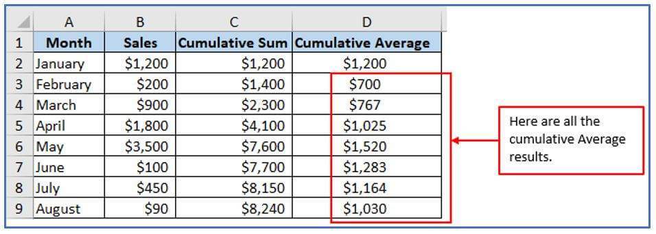
 3.How to use the scanning function Cumulative Average in Excel?
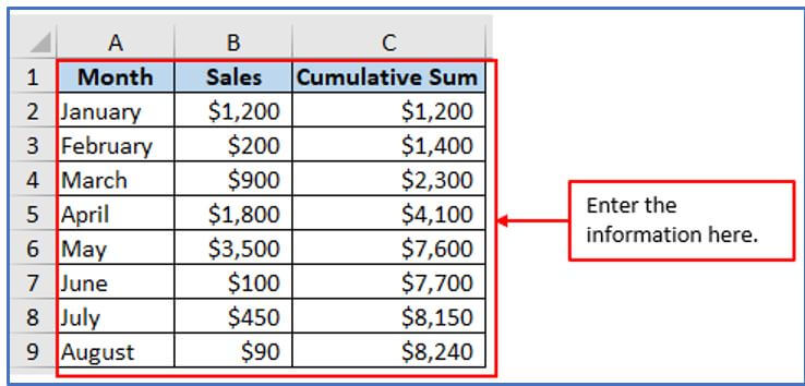
Step 1: Make a dataset with the information as shown below.
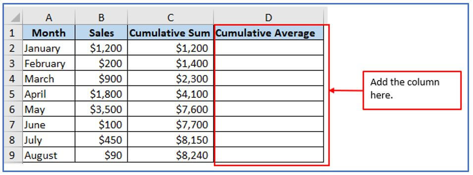
Step 2: Now you need to add the column in D1:D9 to get the Cumulative Average result there.
Step 3: Now use the formula. The formula: =SCAN(0,B2:B9,LAMBDA(a,b,a+b))/SEQUENCE(COUNTA(C2:C9))
Here, the sequence is the column range.

Step 4: Press enter and the result will come out.
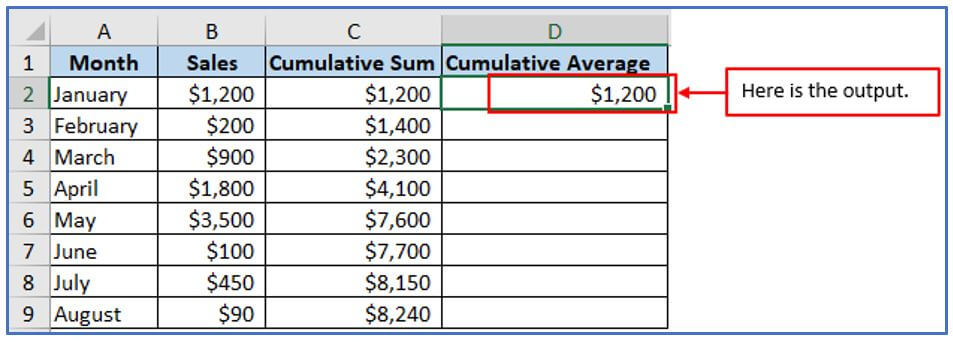
Step 5: Now use the same formula or drag-down the cursor to get the all outputs.
4. How to use the scanning function Cumulative Max in Excel?
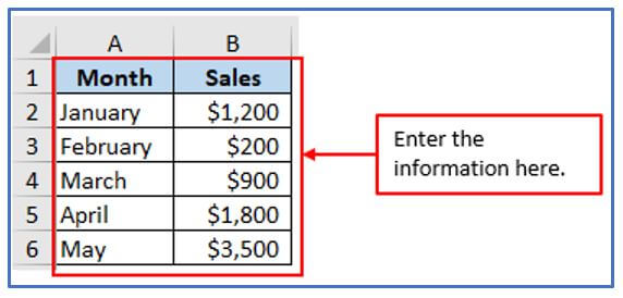
Do make an example like the below picture where have two lists Month and sales.
Step 1: First make a list by writing the month names and sales and enter that data into the table.
Step 2: Now, make another table starting in cell D1:D6 to get the Cumulative Max
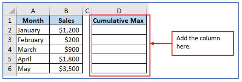
Step 3: It always starts with initial value. Now, use the Cumulative MAX formula. =SCAN(0,B2:B6,LAMBDA(a,b,MAX(a,b)))

Step 4: Press enter and the result will come out. Use the MAX function to calculate the maximum value between the two. Accumulator (a) corresponds to the previous output of the LAMBDA function. The value parameter (b) is equal to the current element of the array. This entire process continues until the last element of the array.

Step 5: Now, use the same formula from Step-3 changing with the column number or drag-down the cursor from C3.
Here are all the cumulative max outputs.

5. Tips for Excel Scan Function in Excel.
To simulate scanning functionality (search for specific data in a range) in Excel, consider the following tips:
- Use conditional formatting: Use conditional formatting to highlight cells that contain the value you’re searching for, resulting in improved visual clarity and identification. This is done by using an alpha-beta function.
- Use filters: Excel’s filter features allow you to quickly narrow down the displayed data within a range based on specific criteria, effectively “scanning” for the information you’re looking for.
- Data Validation Dropdown List: Using the “optional” data validation dropdown list, users can choose from a variety of options to validate their cell entries and reduce errors.
- VLOOKUP or INDEX/MATCH: By using VLOOKUP and INDEX/MATCH, it is possible to search for information in a table and retrieve the appropriate value by specifying criteria.
- Wildcard characters: When using functions such as FIND, SEARCH, VLOOKUP, and MATCH, use wildcard characters (*, ?) to represent unknown characters or patterns for greater search flexibility.
- Named ranges: By defining named ranges for your data, it makes it easier to reference specific ranges in the formula and reduces the likelihood of errors.
- Conditional expressions: Depending on whether the value you are seeking is found, use different actions and provide unique responses using IF statements or other conditional expressions.
- Advanced Filters: Use Excel’s advanced filtering features to perform more complex filtering operations, such as filtering by multiple conditions or extracting unique records.
- Excel Spreadsheet: Converting a data range to an Excel spreadsheet allows for dynamic filtering, sorting, and browsing of data, improving the efficiency of scanning operations.
- Regular Expressions (VBA): Advanced users should consider using Visual Basic for Applications (VBA) to create custom scan functions using regular expressions to provide advanced search functionality.
Using these tips and Excel’s built-in features, you can effectively simulate scan functions that search for specific data in an Excel workbook.
You may be interested:
