Text to Column – Multiple ways to Split Text to Column in Excel

Split Text to Column in Excel is a crucial feature for anyone looking to enhance their data organization and analysis. By mastering this tool, you can transform cumbersome, mixed data into structured, easy-to-analyze formats, streamlining your workflows and uncovering insights more quickly. Whether you’re reformatting imported data, segregating names and addresses, or preparing reports, the ability to split text into columns is indispensable. Embrace this function to make your Excel spreadsheets more versatile and your data manipulation tasks more efficient.

This Tutorial Covers:

1. Text to Columns in Excel: Where to Find Them
   • Example 1 – Split first and last names in names
   • Example 2 – Split email addresses by username and domain name
   • Example 3 – from the URL, obtain the Root Domain
   • Example 4 – Transform Unreliable Date Formats Into Reliable Date Formats
   • Example 5 – Convert Text to Numbers
   • Example 6 – Extract First five Characters of a String
   • Example 7 – Negative integers from numbers with a trailing minus sign

1. Text to Columns in Excel: Where to Find Them

To access Text to Columns, select the dataset and go to “Data” tab and then click “Text to Columns” under “Data Tools” section.

The Convert Text to Columns Wizard would then be displayed.

Before dividing the text into columns, this wizard goes through three steps and requests feedback from the user (you will see how these different options can be used in the examples below).

You may also use the keyboard shortcut ALT + A + E to get to Text to Columns.

Let’s get started and explore some incredible things you can do in Excel with Text to Columns.

• Example 1 – Split first and last names in names

With Excel’s Text to Columns feature, you can easily divide text values into different cells in a row.

Consider the following dataset as an example. Suppose you want to split the first and last names and obtain them in different cells.

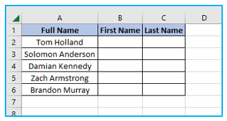
The procedures for utilizing Text to Columns in Excel to separate the first and last names are described below:

Step 1: Choose every name in the column (A2:A6 in this example)

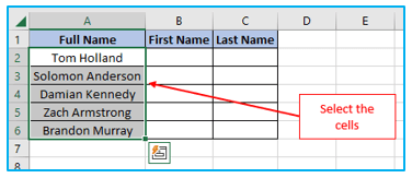
Step 2: Toggle to the “Data” tab. Select the “Text to Columns” option under the “Data Tools” group.

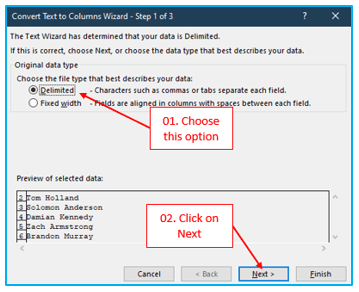
Step 3: The “Convert Text to Column Wizard” dialog box will appear. Click “Next” after choosing “Delimited” (which enables you to use a space as the separator).

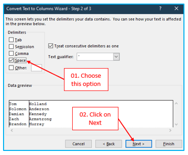
Step 4: Click “Next” after selecting the “Space” option.

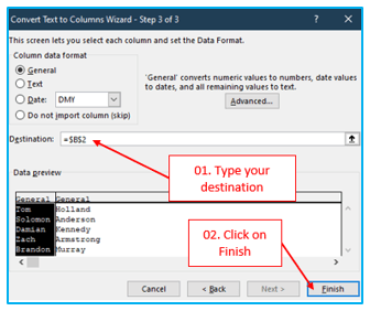
Step 5: Make B2 the final destination cell (else it will overwrite the existing data). Select “Finish”.

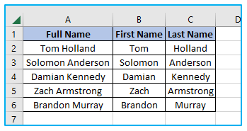
Following the procedures above would immediately separate the names into first and last names (with first names in column B and last name in column C).

Note:

• When your name solely consists of your first and last names, this strategy works effectively. This might not work if there are initials or middle names.
• When you use the Text to Columns tool, you receive a static output. This implies that in order to obtain updated results in the event that the original data changes, you will need to repeat the procedure.

• Example 2 – Split email addresses by username and domain name

You can select your own delimiter to split text using Text to Columns.

Since usernames and domain names are separated by the @ symbol, this can be used to divide email addresses into usernames and domain names.

Assume you have the dataset as follows:

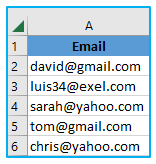
Here are the steps for using the Text to Columns function to separate these usernames and domain names.

Step 1: Choose the whole data set except the header.

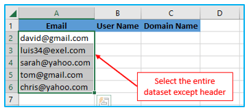
Step 2: Toggle to the “Data” tab. Select the “Text to Columns” option under the “Data Tools” group.

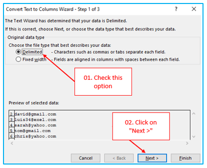
Step 3: Ensure that “Delimited” is chosen (which is also the default selection). Select Next.

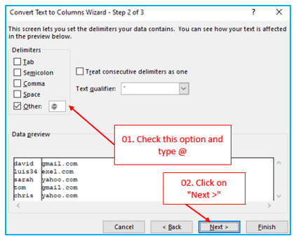
Step 4: In the box to the right of “Other,” type @. Make sure to uncheck every alternative (if checked). Select Next.

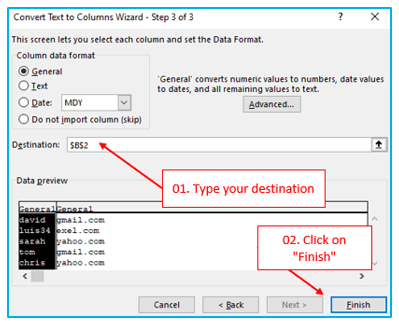
Step 5: The cell where you want the outcome should be the new destination cell. Select Finish.

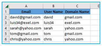
The first name and last name would be provided to you in different cells along with a split email address.

• Example 3 – from the URL, obtain the Root Domain

If you work with online URLs, you might occasionally need to know how many different root domains there are.

For instance, the root domain, www.google.com, is the same for both http://www.google.com/example1 and http://google.com/example2.

Assume you have the dataset as follows:

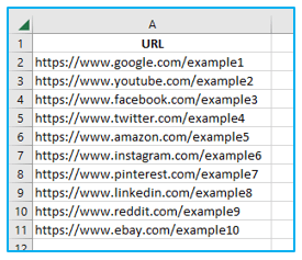
The steps to extract the root domain from these URLs are as follows:

Step 1: Choose the whole data set except the header.

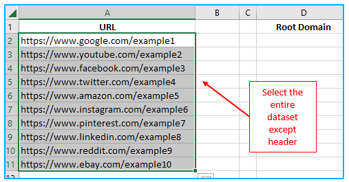
Step 2: Toggle to the “Data” tab. Select the “Text to Columns” option under the “Data Tools” group.

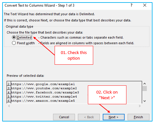
Step 3: Ensure that “Delimited” is chosen (which is also the default selection). Select Next

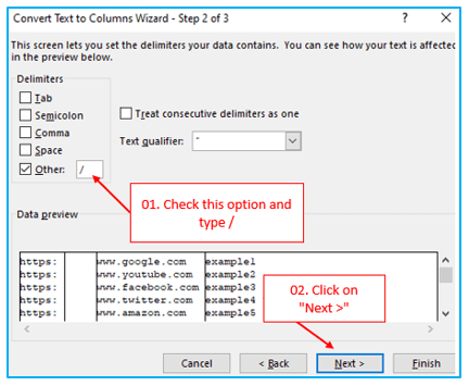
Step 4: Choose Other, then type “/” (a forward slash) in the box next to it. Make sure to uncheck every alternative (if checked). Select Next.

Step 5: The cell where you want the outcome should be the new destination cell. Select Finish.

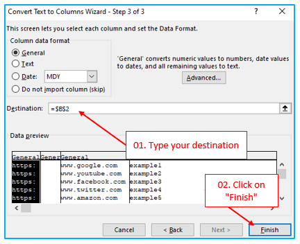
By doing this, you may break up the URL and get the root domain (in the third column as there were two forward slashes before it).

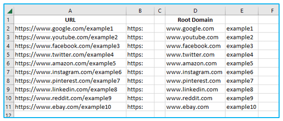
Now, just eliminate the duplicates to determine the number of unique domains.

Note: When all of your URLs start with http://, this will function properly. If not, the root domain will be displayed in the first column by itself. Making these URLs consistent before using Text to Columns is a smart idea.

• Example 4 – Transform Unreliable Date Formats Into Reliable Date Formats

There is a chance that the date format will be inaccurate if you import your data from a text file or obtain it from databases like SAP/Oracle/Capital IQ.

Excel only supports a small number of file types; any other file format must be converted before it can be used in Excel.

Assume that your dates are in the following format (which are not in the valid Excel date format).

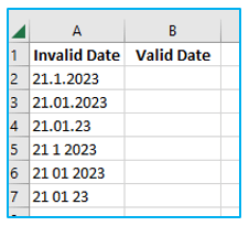
The steps to change these into acceptable date formats are as follows:

Step 1: Choose the whole data set except header.

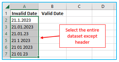
Step 2: Toggle to the “Data” tab. Select the “Text to Columns” option under the “Data Tools” group.

Step 3: Ensure that “Delimited” is chosen (which is also the default selection). Select Next

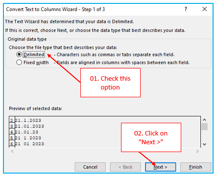
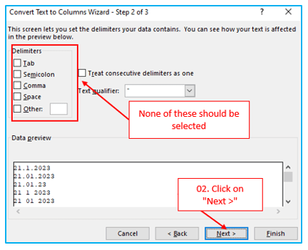
Step 4: Ensure that the NO delimiter option is chosen. Select Next.

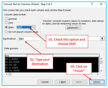
Step 5: Choose Date in the Column Data Format and then the desired format (DMY would mean date month and year). Click on Finish.

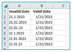
These erroneous date formats would be instantaneously converted into legitimate date forms that you may use in Excel.

• Example 5 – Convert Text to Numbers

The numbers are occasionally transformed into text representation when you import data from databases or other file formats.

There are various methods for this to occur:

• The number comes before an apostrophe. As a result, the number is handled as text.
• Using text functions like LEFT, RIGHT, or MID to generate numbers

The issue with this is that Excel functions like SUM and AVERAGE ignore these numbers (which are in text format).

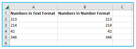
Consider the following dataset, where the numbers are presented in text format (note that these are aligned to the left).

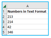
To convert text to numbers using Text to Columns, follow these steps:

Step 1: Choose the whole data set except header.

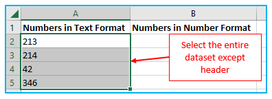
Step 2: Toggle to the “Data” tab. Select the “Text to Columns” option under the “Data Tools” group.

Step 3: Ensure that “Delimited” is chosen (which is also the default selection). Select Next

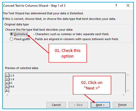
Step 4: Ensure that the NO delimiter option is chosen. Select Next.

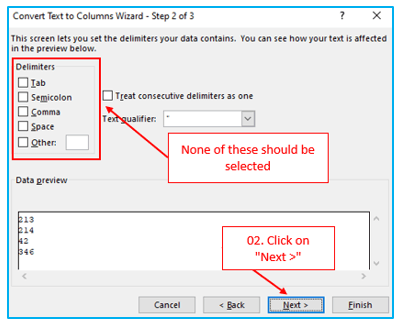
Step 5: Select “General” from the Column data format menu. Change the destination cell as well to the one where you want the outcome to appear. Select Finish.

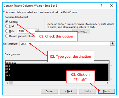
By doing this, these numbers would once again be in General format and be used in formulas.

• Example 6 – Extract the First five Characters of a String

It’s occasionally necessary to remove the first few characters from a string. The first five characters (or any other number of characters) in transactional data that serve as a unique identifier may be the case in these situations.

For instance, the first five letters in the data set below are specific to a product line.

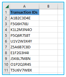
Using Text to Columns, use these steps to quickly extract the first five characters from this data:

Step 1: Choose the whole data set except header.

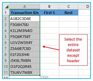
Step 2: Toggle to the “Data” tab. Select the “Text to Columns” option under the “Data Tools” group.

Step 3: make certain “Fixed Width” is chosen. Select Next.

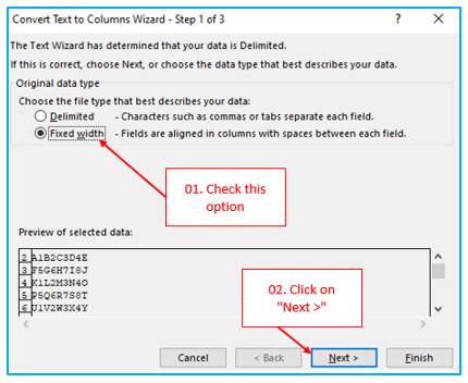
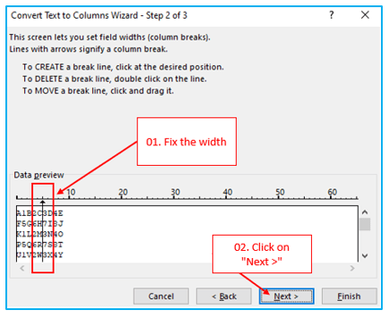
Step 4: Drag the vertical line to the fifth character in the text after which it will be placed in the Data preview area. Select Next.

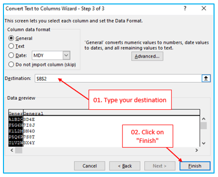
Step 5: The cell where you want the outcome should be the new destination cell. Select Finish.

By doing this, your data set would be divided, giving you the first five characters of each transaction id in one column and the remaining characters in the second.

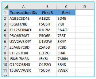
Note: To divide the data into more than two columns, you can also set up additional vertical lines. To set the divider, simply click and drag the mouse anywhere within the Data Preview window.

• Example 7 – Negative integers from numbers with a trailing minus sign

Even while you might not run into this very often, you could occasionally need to make the numbers negative by adding the following minus signs.

The best solution for this is Text to Columns.

Assume you have the dataset as follows:

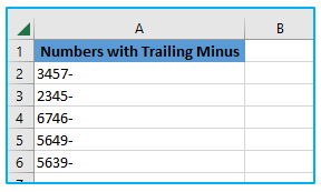
These trailing minuses can be turned into negative numbers by following these steps:

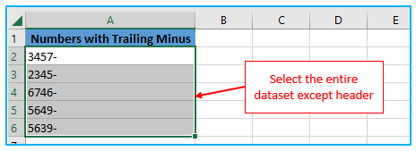
Step 1: Choose the whole data set except header.

Step 2: Toggle to the “Data” tab. Select the “Text to Columns” option under the “Data Tools” group.

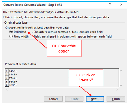
Step 3: Ensure that “Delimited” is chosen (which is also the default selection). Select Next

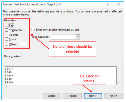
Step 4: Ensure that the NO delimiter option is chosen. Select Next.

Step 4: Select “Advanced” from the menu.

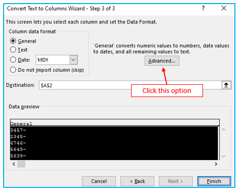
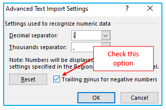
Step 5: Pick the “Trailing minus for negative numbers” option in the Advanced Text Import Settings dialog box. Select OK.

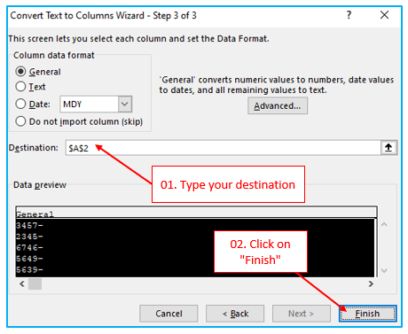
Step 6: Decide on the final cell. Select Finish.

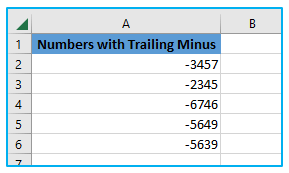
This would immediately move the negative sign from the beginning to the end of the number. These figures are now simple to utilize in computations and formulas.

Application of Split Text to Column in Excel

For ready-to-use Dashboard Templates:

1. Financial Dashboards
2. Sales Dashboards
3. HR Dashboards
4. Data Visualization Charts