The NPER function in Excel, short for “Number of Periods,” is a powerful tool for financial analysis and planning. This function is especially valuable when it comes to making critical financial decisions, such as loan or investment planning. NPER allows users to determine the number of payment periods required to reach a specified financial goal, taking into account factors like interest rates, regular contributions or withdrawals, and the present value of an investment. Whether you’re working on retirement planning, evaluating a loan, or estimating the time needed to reach a savings target, understanding how to use the NPER function can simplify complex financial calculations and help you make informed decisions with confidence. In this guide, we will explore the ins and outs of the NPER function, demonstrating its practical applications and showing you how to use it effectively in various financial scenarios.
This content Covers:-
- What is NPER Function?
- Using NPER function in Excel with formula
- Apply NPER function in Excel
- Apply Basic NPER formula in Excel
- How to use NPER function in Excel ?
- Calculate the number of periodic payments for a loan
- Calculate NPER based on present and future values
1. What is NPER Function?
“NPER” stands for “Number of Periods.” Basically, It is based on a fixed interest rate, periodic payment amount and the current or future value of the loan or investment. NPER(Number of periods) helps you determine how long it will take to reach a specific financial goal or pay off debt by indicating the number of periods needed.
This function is often used in financial planning, such as to calculate the term of a loan or the time needed to reach a savings goal.
In the below example here is given, Loan amount, monthly payment and yearly interest rate, so calculate the Rate of Interest (ROI).

2. Using NPER function in Excel with formula ?
The NPER function uses the following arguments:
Interest rate (required) – Interest rate per period. If you make payments once a year, specify an annual interest rate; If you pay monthly, indicate the monthly interest rate, etc.
Pmt (required argument) – The payment made each period. Typically, it includes principal and interest but no other fees or taxes.
Pv (required argument) – The present value or gross amount that a series of future payments is currently worth. That is, the present value of a series of future cash flows.
Fv (optional argument) – This is the future value or cash balance we want at the end after the last payment. When omitted, it takes on a value of 0.
Type (optional argument) – Indicates when payment is due. If type is set to 0 or omitted, payments are due at the end of the period.
If the value is 0,
then payment is due at the beginning of the period.
If the value is 1,
the beginning of the accounting period
Step 1: Insert the Data into your excel sheet.
Entering the Data.

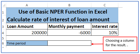
Step 2: Now, choose a column for getting the result of the rate of interest of the loan amount there.
You can see a column A6 is selected below and named it time period for getting ROI(rate of interest).
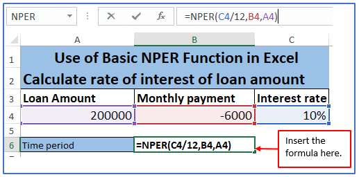
Step 3: Now, insert the formula according to your information column.
Formula: =Nper (D4/12, C4,B4), in here interest rate is given yearly But the payment method is given monthly, so the interest rate turned into monthly. That’s why the interest rate is divided by 12.
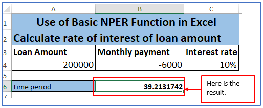
Step 4: After entering the formula Press enter.
Here is the result of rate of interest below.
3. Apply NPER function in Excel
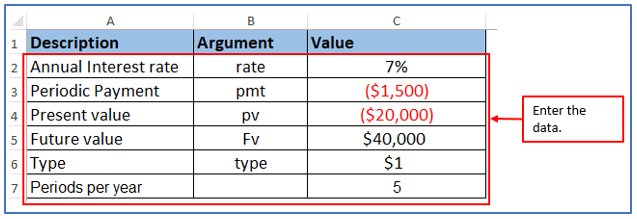
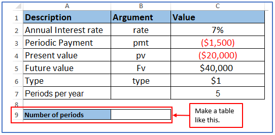
Step 1: First, take some information and put them into excel.
Where,
- Annual interest rate (rate) – 7%
- Periodic payment (pmt) – -$1500
- Present value (pv) : -$20,000
- Future value (fv) – 40,000
- When payments are due (type) – 1
- Periods per year – 5
- What is the number of periods?
Entered the above data into an Excel sheet.
Step 2: Now, Choose any one column for extracting the results.
Choosing A9 and B9 for receiving the result.
Step 3: To get the exact periodic interest rate, the annual interest rate (C2) is divided by the number of periods in the year (C7).
The formula is: =NPER(C2/C7,C3,C4,C5,C6)
Use the formula below.
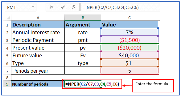
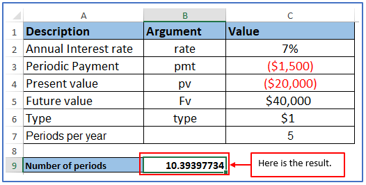
Step 4: When the formula is set, press enter and the result will come out.
Here is the result below:
4. Apply Basic NPER formula in Excel
Here are some basic steps to better understand Knope theory in its simplest form to get the number of loan payment periods based on the following data:
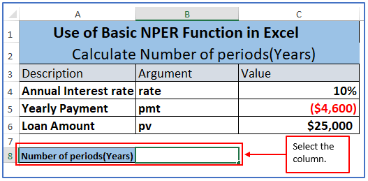
Step 1: Put this data in you excel as written.
Annual interest rate (interest rate): 10%
Annual payment (pmt): -$4600
Loan amount (pv): $25,000

Step 2: Now, choose a column for getting the result of the rate of interest of the loan amount there.
You can see a column A8 and B8 is selected below and named it Number of periods(Years) to get the result.
Step 3: Now you can use this basic formula to calculate the number of periods.
=NPER(C4,C5,C6)
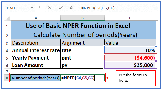
Step 4: After entering the formula, you need to press Enter. After pressing Enter you will get the results as shown below.
In this case, the future value(FV) is not relevant and is ignored since the payment is due at the end of the year, which is the default type.
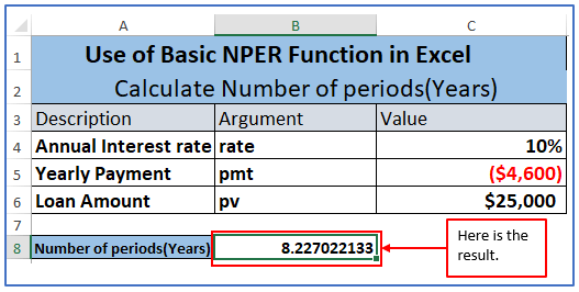
Step 5: Here, You are offered a loan of $25,000 at 10% annual interest, and you pay $4,600 to the bank each year. This formula indicates that it will take eight payments per year to repay the loan.
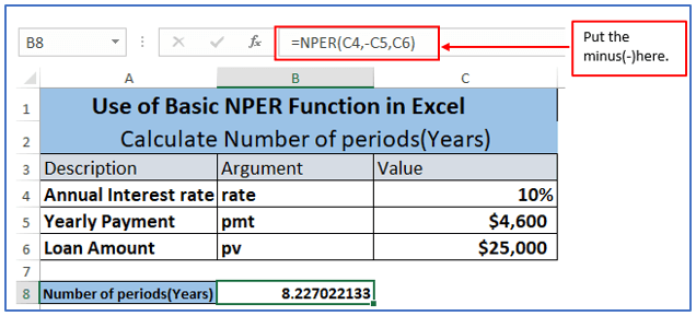
If you want to enter the recurring payment as a positive number, insert a minus sign directly before the PMT argument in the formula as the picture shows.
=NPER (C4,-C5,C6)
5. How to use the NPER function in Excel?
5.1 Calculate the number of periodic payments for a loan
Most of the loans and long-term loans are repaid in monthly installments. Some are paid quarterly or semi-annually. For calculating this type of loan thing is to convert the annual interest rate to a periodic interest rate. You need to divide the annual percentage rate by the number of periods in the year. To do this, the formulas are:
For, Monthly payments: rate = annual interest rate / 12
For, Quarterly payments: rate = annual interest rate / 4
For, Semiannual payments: rate = annual interest rate / 2
Example:
You can start by entering data into the cells following the underneath picture:
Annual interest rate : 6%
Yearly Payment (pmt): $700
Loan amount (pv): $20,000
Step 1: Put the information into the table.
Entered the information here.

Step 2: Now, choose a column for getting the result of the rate of interest of the loan amount there.
You can see a column A8 and B8 is selected below and named it Number of periods(Monthly) to get the result.
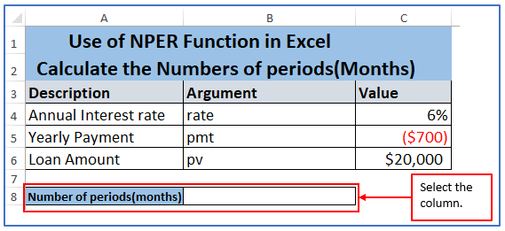
Step 4: Divide C4 by 12 and follow the formula to calculate the number of monthly payments on the loan:
=NPER(C4/12,C5,C6)
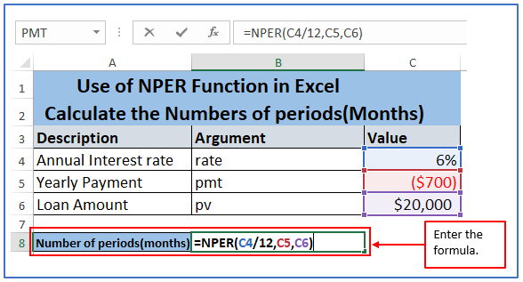
Step 5: Now press Enter and the result will come out.
The result is outlined below. After seeing the result the photo says that it will take 30 months or (2 year 6 months) to pay off.
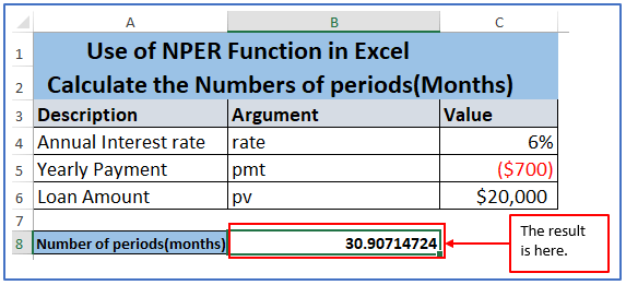
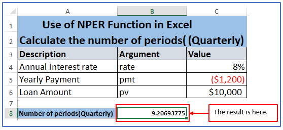
Step 6: For Quarterly, You can start by entering data into the cells following the underneath picture:
Annual interest rate (C2): 8%
Monthly Payment (Pmt): $1200
Loan amount (Pv): $10,000
What is the periods of number quarterly?

Step 7: Now, choose a column for getting the result of the rate of interest of the loan amount there.
You can see a column A8 and B8 is selected below and named it Number of periods(Quarterly) to get the result.
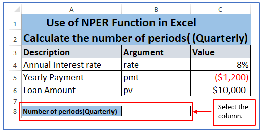
Step 8: Using F4/4 for rate for NPER to return periods in quarters. The formula is:
=NPER(C4/4,C5,C6)
The formula is used below.
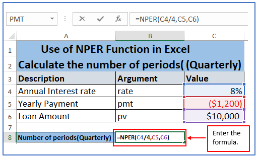
Step 9: Now, press Enter and the answer will show.
The result is outlined below:
5.2 Calculate NPER based on present and future values
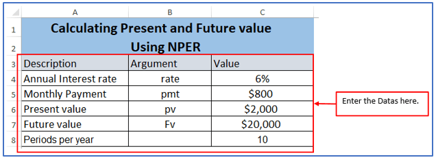
Step 1: For calculating NPER based on present and future values, first pick some data and enter into the excel.
Where,
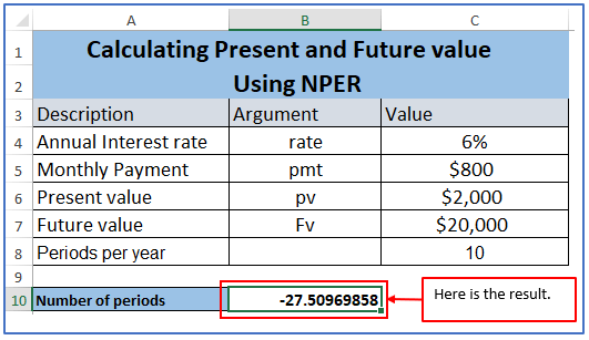
- Annual interest rate : 6%
- Monthly payment (pmt) : -800
- Present value(pv) : -2,000
- Future value (Fv): 20,000
- Periods per year : 10
- Calculate the number of periods.
Entered the datas.
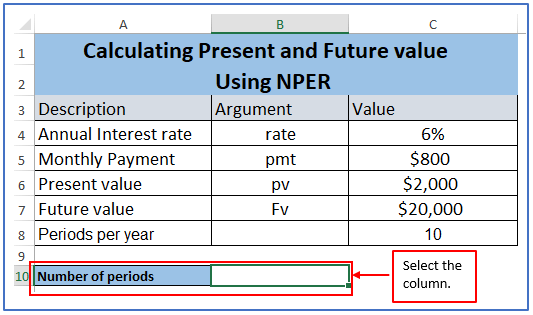
Step 2: Now, choose a column for getting the result of the rate of interest of the loan amount there.
You can see a column A10 and B10 is selected below and named it Number of periods(Quarterly) to get the result.
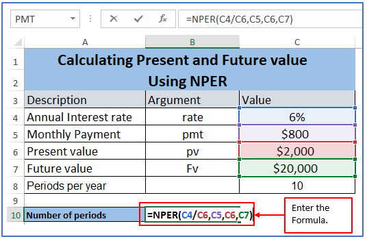
Step 3: For this the formula will be: =NPER(C4/C6,C5,C6,C7)
In the below picture, the formula is entered.
Step 4: The result is here and it is negative. That means the investment will not be profitable.
You may be interested:
