Microsoft 365 is the latest and upgraded version of Microsoft Excel. This new and upgraded version has a large number and variety of functions and formulas added in it for better use of its users. In this tutorial, we will see and know about some of the new formulas of Microsoft 365, their functions, and how to use them.
This Content Covers:
- ARRAYTOTEXT Formula
- BYCOL Formula
- BYROW Formula
- CHOOSECOLS Formula
- CHOOSEROWS Formula
- DROP Formula
- EXPAND Formula
- FIELDVALUE Formula
- HSTACK Formula
- ISOMITTED Formula
- ARRAYTOTEXT Formula
Purpose of the Function
The purpose of ARRAYTOTEXT function is to return an array of text values from a specified range of cells and columns. While returning an array of texts, it keeps the text values unchanged and converts the not-text values into texts.
Function Syntax and Arguments
Syntax:
ARRAYTOTEXT(array,[format])
Arguments
- The formula has to return the array as text.
- The format of the returned data can be of two values either 0 or 1. Here 0 is for concise and 1 for strict.
Examples and Output Result (including suitable data set and table)
Both the format values will be applied in this dataset to see if they return as text values or not.

0/Concise: Select cell C1 and insert the formula given in the picture below and click ENTER.

1/Strict: Enter this formula in cell C1 and press ENTER.

Explanation of Output Result
The concise (0) formula returned the text values unchanged from the selected range.
The Strict (1) formula returned the text values with quotation marks applied on each of the values separately from the selected range.
Both the formulas changed the value of cell A3 from a non-text value to text value.
- BYCOL Formula
Purpose of the Function
The purpose of BYCOL function is to return one result per column as a single array after applying a LAMBDA function to each column in the specified array.
Function Syntax and Arguments
Syntax:
=BYCOL(array, lambda(column))
Arguments:
- An array with column separation.
- The LAMBDA function to be applied in each column but will calculate only one result.
- A column from an array.
Examples and Output Result (including suitable data set and table)
Here we have a range of values in which we have to apply the BYCOL formula.
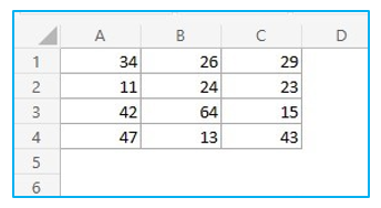
Example 1: Select cell E1>>insert the formula in the picture and hit ENTER.
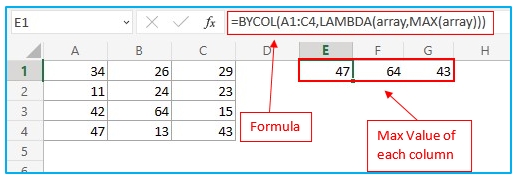
Example 2: Type the formula in E1 and press ENTER key.

Example 3: Inset the formula in cell E1 and click ENTER.
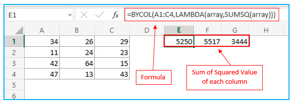
Explanation of Output Result
The formula in Example 1 returns the maximum/highest value of each column using MAX function and Example 2 returns the minimum value of each column using MIN function.
The formula in Example 3 uses SUMSQ function and returns the sum of the squared value of each array element in each column.
- BYROW Formula
Purpose of the Function
The purpose of BYROW function is to return one result per row as a single array after applying a LAMBDA function to each row in the specified array.
Function Syntax and Arguments
Syntax:
=BYROW(array, lambda(row))
Arguments:
- An array with row separation.
- The LAMBDA function to be applied in each row but will calculate only one result.
- A row from an array.
Examples and Output Result (including suitable data set and table)
In this case, we will use the BYROW formula on this set of values.
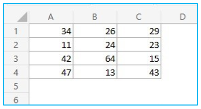
Example 1: Type the formula in E1 and press ENTER key.
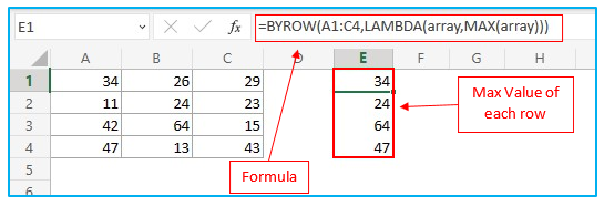
Example 2: Select cell E1>>insert the formula in the picture and hit ENTER.
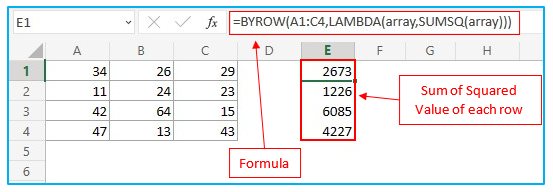
Explanation of Output Result
Example 1 returns the maximum/highest value of each row using MAX function.
The formula in Example 2 returns the sum of the squared value of each array element in each row using SUMSQ function.
- CHOOSECOLS Formula
Purpose of the Function
The purpose of CHOOSECOLS function is to return specified columns from an array.
Function Syntax and Arguments
Syntax:
=CHOOSECOLS(array,col_num1,col_num2….)
Arguments:
- The array that contains the columns will be returned in the new array.
- The first column has to be returned as this is compulsory.
- Additional columns also will be returned, not compulsory.
Examples and Output Result (including suitable data set and table)
Example 1: Insert the formula in the picture below in cell E1 and click ENTER.
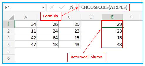
Example 2: Choose cell E1 and type the formula inside this cell. Hit ENTER.

Explanation of Output Result
The formula in Example 1 returns the chosen column (col 3) in cell E1. The formula returns only one column here as we put the serial number of only column 3.
In Example 2, we have selected the columns serial number as 2,1,3,1. The formula returns these specified columns in this order. We also can see column 1 appearing twice as we have chosen column 1 in two occasions in the formula.
- CHOOSEROWS Formula
Purpose of the Function
The purpose of CHOOSEROWS function is to return specified rows from an array.
Function Syntax and Arguments
Syntax:
=CHOOSEROWS(array,row_num1,row_num2…..)
Arguments:
- The array that contains the rows will be returned in the new array.
- The first row has to be returned as this is compulsory.
- Additional rows also will return, not compulsory.
Examples and Output Result (including suitable data set and table)
Example 1: Insert the formula given in below picture in cell E1 after selecting it. Press ENTER key.
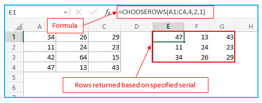
Explanation of Output Result
In Example 1 we have selected the serial of rows as 4,2,1 so the formula has returned the specified rows according to this serial. Row 3 is not returned here because we did not specify it inside the formula.
- DROP Formula
Purpose of the Function
The DROP formula’s purpose is to prevent a certain number of rows or columns from being included at the beginning or end of an array.
Function Syntax and Arguments
Syntax:
=DROP(array, rows,[columns])
Arguments:
- The array or range from which the rows and columns will be dropped.
- The quantity of rows to remove. A negative value will drop rows from the end of an array.
- The number of columns to drop. A negative value will drop columns from the end of an array.
Examples and Output Result (including suitable data set and table)
We will apply the DROP formula in this datasheet to see how the formula works.
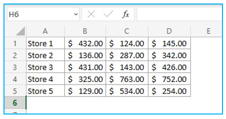
Example 1: Select cell F1 and insert the formula given in the below picture. Click ENTER.

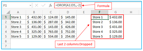
Example 2: Insert the formula from the below given picture in cell F1 and hit ENTER key.

Example 3: Type the formula in F1 after selecting this cell and press ENTER.
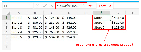
Example 4: Click on cell F1>>insert the formula>>press ENTER.
Explanation of Output Result
Example 1 drops or removes the first three rows as we selected 3 in the formula which indicates the number of rows that will be dropped.
In Example 2 we used two comas ( ,, ) and select 2 as the number of columns that should be removed or dropped. These double comas enable the formula to be applied for columns instead of rows. As we selected 2 inside the formula, the first two columns have been dropped.
We used a minus ( – ) value in Example 3 which dropped the last two columns from the array.
Example 4 drops first two rows and last two columns as we selected a positive and a negative value inside the formula ( 2,-2 ).
- EXPAND Formula
Purpose of the Function
The purpose of EXPAND formula is to expand or pad an array to the given number of rows and columns.
Function Syntax and Arguments
Syntax:
=Expand(array, rows, [columns], [pad_with])
Arguments:
- An array or a range to expand.
- The expanded array’s total number of rows. Rows won’t be expanded if they are missing.
- The expanded array’s total number of columns. Columns won’t be expanded if they are missing.
- The default value to pad with is #N/A which is changeable.
Examples and Output Result (including suitable data set and table)
Example 1: Select cell F1 and insert the formula in that cell. Hit ENTER.

Example 2: Type the formula in cell F1 after selecting it and press ENTER key.

Explanation of Output Result
Example 1 resizes a 5X4 array to a 6X6 array and pad empty elements with #N/A.
Example 2 resizes a 5X4 array to a 6X5 array and pads empty elements with “-” as we selected (“-“) inside the formula.
- FIELDVALUE Formula
Purpose of the Function
The purpose of FIELDVALUE formula is to obtain field data from linked data types like Stocks or Geography data types etc. The FIELDVALUE function should primarily be used to create conditional calculations using linked data types.
Function Syntax and Arguments
Syntax:
=FIELDVALUE(value, field_name)
Arguments:
- When given a linked data type as the value parameter, the function returns any matching fields from that data type.
- The name(s) of the field(s) from the linked data type that you want to extract.
Examples and Output Result (including suitable data set and table)
Example 1: Select cell C3 and insert the formula from the picture below, hit ENTER. Click and drag the lower right corner of C3 to D3 to apply the formula in that cell too.

Example 2: Insert the formula shown below in cell C3>>press ENTER>>click and drag C3 to D3.

Explanation of Output Result
The formula =FIELDVALUE(A2,”Price”) in Example 1 extracts the Price Field for MICROSOFT CORPORATION (XNAS:MSFT). The same formula returns a #FIELD error in cell D3 as it could not find the field value.
To get rid of the #FIELD error from Example 1, we have used IFERROR with FIELDVALUE formula in Example 2 to change the error text to ( – ) if the formula doesn’t find the field value.
- HSTACK Formula
Purpose of the Function
The purpose of HSTACK formula is to combine many smaller arrays into one bigger array by appending them horizontally and in order.
Function Syntax and Arguments
Syntax:
=HSTACK(array1,[array2],…)
Arguments:
- The highest number of rows from each array parameter.
- The total number of columns from every array parameter.
Examples and Output Result (including suitable data set and table)
Example 1: Insert the formula in J2 after selecting it and press ENTER.

Example 2: Click on ENTER button after selecting and inserting the formula from the below picture in cell J1.

Explanation of Output Result
The formula in Example 1 horizontally appends two simple arrays in sequence so that the results are one array.
In Example 2, the formula horizontally appends three simple arrays in sequence so that the results are one array. Cell G2 is empty so the formula returns a 0 in the combined array in cell N2 instead of a blank cell.
- ISOMITTED Formula
Purpose of the Function
The purpose of ISOMITTED formula is to check whether the value in a LAMBDA is missing and returns TRUE or FALSE.
Function Syntax and Arguments
Syntax:
=ISOMITTED(argument)
Arguments:
- The value you wish to test, like a LAMBDA parameter.
Examples and Output Result (including suitable data set and table)
Example 1: Select cell A1 and insert the formula shown in the picture. Press ENTER key.

Explanation of Output Result
The formula in Example 1 has checked for a missing parameter and returned a friendly string.
You may be interested:
