Microsoft 365 Excel New Formula in 2022 and 2021: Part 2

Microsoft has made a ton of modifications to Excel over the last few years.

The cool new upgrades to Excel for Windows, Mac, the web, and mobile devices will all help us do our work more quickly. This covers a wide range of topics, from brand-new keyboard shortcuts to sophisticated (Lambda) functions for intricate array calculations.

In this tutorial, you will learn Microsoft 365 New formulas in 2022 and 2021 named LAMBDA, MAKEARRAY, MAP, REDUCE AND SCAN.

This Tutorial Covers:

1. LAMBDA Function
   • Purpose of the function
   • Syntax
   • Arguments
   • Explanation a LAMBDA Function with Example
   • Explanation of output result
2. MAKEARRAY Function
   • Purpose of the function
   • Syntax
   • Arguments
   • Explanation a MAKEARRAY Function with Example
   • Explanation of output result
3. MAP Function
   • Purpose of the function
   • Syntax
   • Arguments
   • Explanation a MAP Function with Example
   • Explanation of output result
4. REDUCE Function
   • Purpose of the function
   • Syntax
   • Arguments
   • Explanation a REDUCE Function with Example
   • Explanation of output result
5. SCAN Function
   • Purpose of the function
   • Syntax
   • Arguments
   • Explanation a SCAN Function with Example
   • Explanation of output result
6. STOCKHISTORY Function
   • Purpose of the function
   • Syntax
   • Arguments
   • Explanation a STOCKHISTORY Function with Example
   • Explanation of output result
7. TEXTAFTER Function
   • Purpose of the function
   • Syntax
   • Arguments
   • Explanation a TEXTAFTER Function with Example
   • Explanation of output result
8. TEXTBEFORE Function
   • Purpose of the function
   • Syntax
   • Arguments
   • Explanation a TEXTBEFORE Function with Example
   • Explanation of output result
9. TEXTSPLIT Function
   • Purpose of the function
   • Syntax
   • Arguments
   • Explanation a TEXTSPLIT Function with Example
   • Explanation of output result
10. TAKE Function
    • Purpose of the function
    • Syntax
    • Arguments
    • Explanation a TAKE Function with Example
    • Explanation of output result

1. LAMBDA Function:

Since you can test every potential combination of inputs and the conditions they effect, it is impossible to achieve unexpected outcomes from your computer programs in traditional programming, where several inputs can alter your output values.

With the help of the LAMBDA Excel function, you can perform some basic programming in Excel and substitute if-then statements with value-only formulas!

• Purpose of the function:

To construct unique, reusable functions that you may call by a familiar name, use a LAMBDA function. The new function has a similar name to native Excel functions and is accessible throughout the entire file.

You can add your own functions to the built-in Excel function library by creating a function for a frequently used formula, doing away with the requirement to copy and paste the formula (which can be error-prone). A LAMBDA function can also be used by non-programmers because it doesn’t require JavaScript, VBA, or macros.

• Syntax:

=LAMBDA([parameter1, parameter2, …,] calculation)

• Arguments:

parameter- A value you want to send to the function, such as a string, number, or cell reference. A maximum of 253 parameters may be entered. This argument is not required.

calculation- The formula you want to run and have the function return as a result. It must be the final argument and must produce a conclusion. This justification is necessary.

• Explanation a LAMBDA Function with Example:

Typically, LAMBDA functions are developed and tested in the worksheet’s formula bar before being placed into the name manager and given a name that may be used throughout the workbook.

A custom LAMBDA function can be created and used in four simple steps:

• Verify your reasoning with a common formula.
• Make and evaluate an unnamed, generic LAMBDA version of the formula.
• Name and describe the manager in the LAMBDA formula.
• Use the specified name to call the new custom function.

These steps are discussed in more detail below.

Step 1: Let’s start with a very basic formula to demonstrate how LAMBDA functions:

=x*y // multiply x and y

This formula commonly uses cell references in Excel that look something like this:

=A2*B2 // with cell references

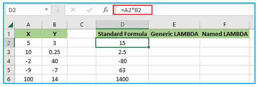
You can see that the formula functions properly, thus we can now proceed to constructing a general LAMBDA formula (unnamed version). The formula’s input requirements should be considered initially (parameters). In this instance, the answer is “yes” because the calculation calls for values for both x and y. With that established, we begin by adding the necessary user input parameters to the LAMBDA function.

=LAMBDA(x,y  // begin with input parameters

Step 2: Next, we must include the calculation itself, x*y:

=LAMBDA(x,y,x*y)

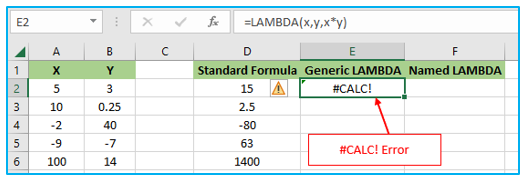
At this point, attempting to enter the formula will result in a #CALC! error. This occurs because there are no longer any cell references, therefore the formula has no input values to deal with.

Step 3: We need to use a particular syntax like this to test the formula:

=LAMBDA(x,y,x*y)(A2,B2) // testing syntax

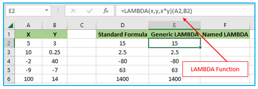
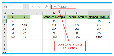
The syntax used at the end of a LAMBDA function, where parameters are supplied in a separate set of parentheses, is exclusive to LAMBDA functions. This enables the formula to be verified before the LAMBDA is named directly on the worksheet. You can see that the generic LAMBDA function in E2 yields the exact same outcome as the original formula in D2 in the screen above.

The LAMBDA function can now be named using the Name Manager.

Step 4: Copy the formula first, omitting the testing settings from the final step.

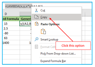
Step 5: After that, click New in the Name Manager by pressing Control + F3.

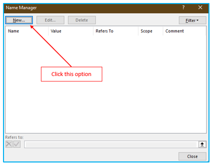
Step 6: Paste the copied formula into the “Refers to” input section of the New Name dialog with the name “XY”, the scope still set to workbook. (Hint: To access the “Refers to” field, use the tab key.)

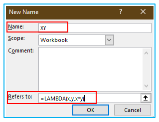
The equals sign (=) should appear at the start of the formula. The LAMBDA formula can be utilized in the workbook just like any other function now that it has a name.

Step 7: Below the copied-down formula in F2 on the screen, we see:

=XY(A2,B2)

• Explanation of output result:

The LAMBDA formula can be utilized in the workbook just like any other function now that it has a name. The old name “=LAMBDA(x,y,x*y)” is replaced with the new name “XY”. To operate with cell references now, there must be input values. The new custom function returns the same result as the previous two formulas when all requirements are satisfied after inputting the formula.

2. MAKEARRAY Function:

Based on a unique LAMBDA calculation, the Excel MAKEARRAY function returns an array with the provided rows and columns. Arrays with changeable dimensions and values that are the outcome of calculations can be made using MAKEARRAY.

• Purpose of the function:

You can quickly create an array (range) of values using MAKEARRAY. The first two arguments should describe the number of rows and columns as well as the expression that the LAMBDA function will use to execute the calculation. Because it returns a range of values that conform to the specified dimensions rather than a single value, this function is similarly dynamic in nature.

• Syntax:

=MAKEARRAY(rows, columns, lambda)

• Arguments:

rows- The array’s total number of rows. should be higher than zero.

cols-How many columns there are in the array. should be higher than zero.

lambda- A call to a LAMBDA that builds the array. The LAMBDA considers two factors:

• row- The row index of the array.
• col- The column index of the array.
• Explanation a MAKEARRAY Function with Example:

In the following formula, MAKEARRAY is used to make a two-by-three array that is filled with the output of multiplying rows by columns:

=MAKEARRAY(2,3,LAMBDA(r,c,r*c))

• Explanation of output result:

The formula returns 1, 2, 3, and 2, 4 and 6.

A “2 x 3” array with the values 1, 2, 3, 2, 4, and 6 is the result.

The result of multiplying rows by columns is used to populate an array with 2 rows and 3 columns.

3. MAP Function:

The MAP function converts each value in the specified array(s) to a new value using a LAMBDA function, and then returns an array.

• Purpose of the function:

Each value in an array is “mapped” by the Excel MAP function to a unique LAMBDA function. Each value receives the LAMBDA treatment, and the output of MAP is an array of results with the same dimensions as the initial array.

• Syntax:

=MAP(array1, [array2], …, lambda)

• Arguments:

array1- The array that will be mapped.

array2- [optional] Additional arrays are needed by the LAMBDA.

lambda- The special LAMBDA function to use.

• Explanation a MAP Function with Example:

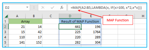
There is an array of data, as the screenshot below demonstrates.

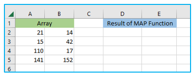
How to use MAP function is shown below:

Step 1: To get the result, paste the formula below into cell D2 and hit Enter.

=MAP(A2:B5,LAMBDA(x, IF(x>100, x*2,x*x)))

• Explanation of output result:

“array1” and “lambda” are the two prerequisite arguments for the MAP function. The array that needs to be mapped is array1 (In this example array1 is “A2:B5”). The specific lambda function named lambda should be used on each element in array1.

The preceding algorithm squares the number in this array when it is less than or equal to 100 and multiplies it by 2 when it exceeds 100.

4. REDUCE Function:

Each member in the specified array is subjected to a specific LAMBDA function by the Excel REDUCE function, which then adds up the results to a single number.

• Purpose of the function:

Applying a LAMBDA to each value in an array reduces it to an accumulated value, which then returns the sum of the values in the accumulator.

• Syntax:

=REDUCE([initial_value], array, lambda)

• Arguments:

initial_value- [optional] the accumulator’s original value.

array- The array that will be shrunk.

lambda- The special LAMBDA function to use

• Explanation a REDUCE Function with Example:

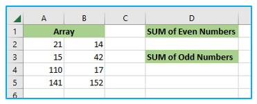
There is an array of data, as the screenshot below demonstrates.

How to use REDUCE function is shown below:

Step 1: Enter the formula below into cell D2 to add the even numbers, and the answer will appear after you press the Enter key.

=REDUCE(0,A2:B5,LAMBDA(a,b,IF(ISEVEN(b),a+b,a)))

Step 2: Enter the formula below into cell D4 to add the odd numbers, and the answer will appear after you press the Enter key.

=REDUCE(0,A2:B5,LAMBDA(a,b,IF(ISODD(b),a+b,a)))

• Explanation of output result:

Initial value, array, and lambda are the three arguments required by the REDUCE function. The initial seed value to use for the ultimate aggregated result is initial value. Initial value is not required. The custom LAMBDA function lambda is applied to each element of the array to determine the final value given by REDUCE. Array is the array to be reduced.

In the two formulations above, “a” stands for the accumulator, which is seeded with the value supplied as initial value to REDUCE, and “b” stands for the various array items. On each entry of the array, the lambda function calculates the total of even and odd numbers. In this example, it returns 318 for the total number of evens and 194 for the total number of odds.

5. SCAN Function:

Applying a LAMBDA to each value in an array allows it to scan the array and return an array containing each intermediate value.

• Purpose of the function:

A custom LAMBDA function is applied to each element in the specified array by the SCAN function, which then returns an array that contains the intermediate values produced during the scan. Running totals and other calculations that display interim results can be produced with SCAN.

• Syntax:

=SCAN([initial_value], array, lambda)

• Arguments:

initial_value- [optional] The accumulator’s initial value.

array- array that will be scanned

lambda- The special LAMBDA function to use

• Explanation a SCAN Function with Example:

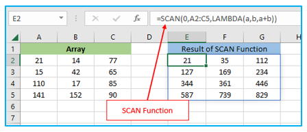
There is an array of data, as the screenshot below demonstrates.

How to use SCAN function is shown below:

Step 1: From column to row, I want to keep adding each value in a cell and its neighboring cell value.

To obtain the result, enter the formula below into cell E2 and hit Enter.

=SCAN(0,A2:C5,LAMBDA(a,b,a+b))

• Explanation of output result:

The accumulator used to produce intermediate values is represented by the first argument, “a”. The initial value supplied to SCAN serves as the starting point for the accumulator, which changes when the SCAN function iterates through the array’s members and performs calculations. The value of each element in the array is represented by the “b” parameter. The calculation is the process that uses a formula to produce the intermediate numbers that will show up in the outcome.

A represents the initial value provided to SCAN (zero) and “b” stands for each unique element in the array in the LAMBDA function. For each element in the array, the LAMBDA runs once, adding the value of “b” to the accumulator each time. The array is the final output of SCAN and is displayed above.

6. STOCKHISTORY Function:

A financial instrument’s historical data is retrieved using the STOCKHISTORY function and loaded as an array, which will overflow if it is the formula’s output. When you press ENTER, Excel will automatically build the proper sized array range.

• Purpose of the function:

Based on a specified symbol and date range, the Excel STOCKHISTORY function returns historical stock price data. Obtaining a financial instrument’s history through time is the main goal of STOCKHISTORY. As a result, a variety of numbers are displayed across several worksheet cells.

• Syntax:

=STOCKHISTORY(stock, start_date, [end_date], [interval], [headers], [properties], …)

• Arguments:

stock- A ticker symbol in quotation marks (“MSFT”, “AAPL”, “GOOG”, etc.).

start_date- The time when the data will first be obtained.

end_date- [optional] The end day on which data can be retrieved. start date is the default.

interval- [optional] Time interval. Monthly = 2, weekly = 1, and daily = 0. Standard is 0.

headers- [optional] Instrument plus header equals 2, while no header equals 0. Standard is 1.

properties- [optional] Further information to be retrieved. Date and Close is the default. Look below.

• Explanation a STOCKHISTORY Function with Example:

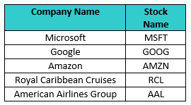
The names of the companies that each stock ticker symbol represents are listed in a small list:

How to use STOCKHISTORY Function is shown below:

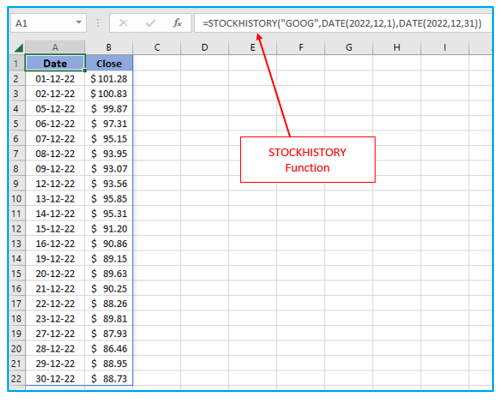
Step 1: For the month of December 2022, enter the following formula in cell A1 to determine the daily close price for Google (“GOOG”):

=STOCKHISTORY(“GOOG”,DATE(2022,12,1),DATE(2022,12,31))

• Explanation of output result:

There is no specified interval, so Daily is used instead (0). Since headers are not given, Date and Close are used by default. The STOCKHISTORY function gives 21 results with this configuration. The first date obtained is December 1, and weekends are not included. Also take note that the start and end dates are provided by the DATE function.

7. TEXTAFTER Function:

Text that follows the specified character or string is returned. It is the TEXTBEFORE function’s inverse.

• Purpose of the function:

The TEXTAFTER function in Excel returns the text that follows a specified delimiter or substring. When there are several delimiters in the text, TEXTAFTER can return text after the nth time a delimiter appears.

• Syntax:

=TEXTAFTER(text, delimiter, [instance_num], [match_mode], [match_end], [if_not_found])

• Arguments:

text- The text string from which to extract.

delimiter- The text’s delimiting character(s).

instance_num- [optional] the text where the delimiter was used. Standard is 1.

match_mode- [optional] Case-sensitivity. 1 indicates a disabled state, whereas 0 indicates an enabled state. Standard is 0.

match_end- [optional] Use the text’s end as a delimiter. 1 indicates that something is enabled; 0 indicates that something is disabled. Standard is 0.

if_not_found- [optional] Value to return in the absence of a match. The default is #N/A.

• Explanation a TEXTAFTER Function with Example:

You must specify the reference to the cell holding the source text for the first parameter (text) and the character enclosed in double quotes for the second argument (delimiter) to extract the text that follows a particular character.

For instance, the following formula will extract text after a space:

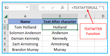
=TEXTAFTER(A2, ” “)

• Explanation of output result:

The above formula’s TEXTAFTER function will return after a space, as shown in the screenshot above.

The first full name is “Tom Holland,” and the TEXTAFTER function returns “Holland” in cell B2 after the second argument.

8. TEXTBEFORE Function:

the text that comes before the specified letter or string is returned. It is the TEXTAFTER function’s inverse.

• Purpose of the function:

The text that comes before a specified substring or delimiter is returned by the Excel TEXTBEFORE function. When a text has several delimiters, TEXTBEFORE might retrieve text prior to the nth instance of the delimiter.

• Syntax:

=TEXTBEFORE(text, delimiter, [instance_num], [match_mode], [match_end], [if_not_found])

• Arguments:

text- The text string from which to extract.

delimiter- The text’s delimiting character(s).

instance_num- [optional] the text where the delimiter was used. Standard is 1.

match_mode- [optional] Case-sensitivity. 1 indicates a disabled state, whereas 0 indicates an enabled state. Standard is 0.

match_end- [optional] Use the text’s end as a delimiter. 1 indicates that something is enabled; 0 indicates that something is disabled. Standard is 0.

if_not_found- [optional] Value to return in the absence of a match. The default is #N/A.

• Explanation a TEXTBEFORE Function with Example:

Suppose you wish to extract the first name that appears before the comma from a list of full names in column A.

This simple formula can be used to accomplish that:

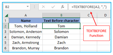
=TEXTBEFORE(A2, “,”)

• Explanation of output result:

The original text string is represented by A2 in the formula above, and the delimiter is a comma (“,”).

The first full name is “Tom, Holland,” and the TEXTBEFORE function returns “Tom” in cell B2 after the second argument.

9. TEXTSPLIT Function:

Column and row delimiters are used to split text strings.

The Text-to-Columns wizard’s functionality is duplicated by the TEXTSPLIT function, but in formula form. You can divide it up by rows or across columns. It is the TEXTJOIN function’s opposite.

• Purpose of the function:

Excel’s TEXTSPLIT function divides text strings into columns or rows based on a specified delimiter. The result is a dynamic array that automatically spills into numerous cells.

• Syntax:

=TEXTSPLIT(text, col_delimiter, [row_delimiter], [ignore_empty], [match_mode], [pad_with])

• Arguments:

text- text string to be divided.

col_delimiter- character(s) used to separate columns.

row_delimiter- [optional] character(s) used to separate rows.

ignore_empty- [optional] Delete any empty values. FALSE = preserve, TRUE = disregard. FALSE is the default.

match_mode- [optional] Case-sensitivity. 1 indicates a disabled state, whereas 0 indicates an enabled state. Standard is 0.

pad_with- [optional] Value for padding 2D arrays with missing values.

• Explanation a TEXTSPLIT Function with Example:

Split text using a substring:

The values in the source string are frequently separated by a string of characters, with a comma and a space serving as an example. Make use of a substring as the delimiter to manage this situation.

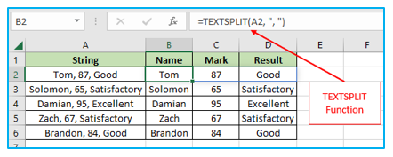
Use the string “, ” for col delimiter, for instance, to use a comma and a space to divide the text in A2 into numerous columns.

=TEXTSPLIT(A2, “, “)

At once, split a string into columns and rows:

You must specify both delimiters in your TEXTSPLIT formula to divide a text string into rows and columns at once.

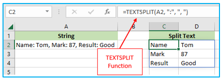
For instance, we offer the following to divide the text string in A2 over columns and rows:

• col_delimiter equal symbol (“:”)
• row_delimiter is a comma and a space (“,”).

The full formula looks like this:

=TEXTSPLIT(A2, “:”, “, “)

• Explanation of output result:

The original text string is represented by A2 in the two formulas above, and the delimiter is a comma (“,”) in the first example and a colon (“:” and “,”) in the second example.

In the first example, the TEXTSPLIT function returns after a specific character named a comma (“,”).

In the second example, the TEXTSPLIT function returns after specific characters named colon (“:”) and comma (“,”), and the outcome is a 2-D array with two columns and three rows.

10. TAKE Function:

a specified number of consecutive rows or columns from the beginning or end of an array are returned.

• Purpose of the function:

A portion of an array is given and returned by the Excel TAKE function. Separate arguments for rows and columns specify the number of rows and columns to return. From either the beginning or the end of the provided array, rows and columns can be removed.

• Syntax:

=TAKE(array, [rows], [col])

• Arguments:

array- The range or source array.

rows- [optional] Returning the number of rows as an integer.

col- [optional] Returning the number of columns as an integer.

• Explanation a TAKE Function with Example:

Suppose you have a dataset like the one below:

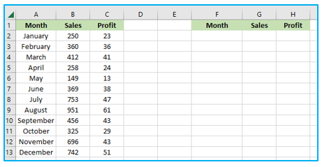
How to use TAKE Function is shown below:

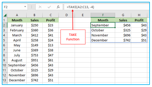
Step 1: The following formula will extract the last four rows from the range A2:C13:

=TAKE(A2:C13, -4)

As many rows and columns as there are in the source range are included in the formula, which starts in cell F2 of the worksheet.

• Explanation of output result:

Provide a positive value for the rows argument to return a specified number of consecutive rows starting at the beginning of a 2D array or range.

Give a negative value for the rows argument to fetch a specific number of rows from the array’s very end.

The rows input in the formula above is a negative number, and the data is taken from the last rows of the range. The formula starts in the range and has as many rows and columns as there are in the source range.

 

You may be interested:

1. Financial Dashboards
2. Sales Dashboards
3. HR Dashboards
4. Data Visualization Charts