Microsoft introduced several new formulas in 2022 and 2021 as in previous years.
The cool new upgrades to Excel for Windows, Mac, the web, and mobile devices will all help us do our work more quickly. This covers a wide range of topics, from brand-new keyboard shortcuts to sophisticated functions for intricate array calculations.
In this tutorial, you will learn Microsoft 365 New formula in 2022 and 2021 named TOCOL, TOROW, VALUETOTEXT, VSTACK, WRAPCOLS, WRAPROWS.
This Tutorial Covers:
- TOCOL Function
- Purpose of the function
- Syntax
- Arguments
- Explanation a TOCOL Function with Example
- Explanation of output result
- TOROW Function
- Purpose of the function
- Syntax
- Arguments
- Explanation a TOROW Function with Example
- Explanation of output result
- VALUETOTEXT Function
- Purpose of the function
- Syntax
- Arguments
- Explanation a VALUETOTEXT Function with Example
- Explanation of output result
- VSTACK Function
- Purpose of the function
- Syntax
- Arguments
- Explanation a VSTACK Function with Example
- Explanation of output result
- WRAPCOLS Function
- Purpose of the function
- Syntax
- Arguments
- Explanation a WRAPCOLS Function with Example
- Explanation of output result
- WRAPROWS Function
- Purpose of the function
- Syntax
- Arguments
- Explanation a WRAPROWS Function with Example
- Explanation of output result
- TOCOL Function:
A column is created out of an array using the Excel TOCOL function. TOCOL may scan data by column in addition to rows, which is how it does by default.
- Purpose of the function:
Excel’s TOCOL function turns a collection of cells into a single column.
- Syntax:
=TOCOL(array, ignore, scan_by_column)
- Arguments:
array- The transformable array.
ignore- The option to ignore mistakes and blanks.
scan_by_column– array by column, scan TRUE = column, FALSE = row (TRUE by default).
- Explanation a TOCOL Function with Example:
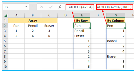
The TOCOL function scans the array horizontally by row when the default scan by column argument (FALSE or omitted) is provided. Set this option to TRUE or 1 to process values by column. For instance:
=TOCOL(A2:C4, ,TRUE)
By Row, type the below formula:
=TOCOL(A2:C4)
- Explanation of output result:
To convert an array into a single column, use the TOCOL function, and to convert it into a single row, use the TOROW function.
In this illustration, a single column is created from three rows and three columns.
The returned arrays in both instances have the same size but distinct value arrangements despite having the same size.
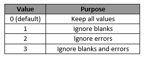
array, ignore, and scan_by_column are the three inputs required by the TOCOL function. The array or range to be changed is represented by the only mandatory argument, Array. The values that TOCOL may choose to ignore are controlled by the ignore argument. The following are the possibilities for ignore:
2. TOROW Function:
A few new functions have been added to Microsoft Excel 365 to conduct various array manipulations. You may quickly do range-to-row transformations with TOROW.
- Purpose of the function:
An array or range is converted into a single row using the TOROW function. Values can be scanned using TOROW’s default row-to-right or column-to-top methods.
- Syntax:
=TOROW(array, ignore, scan_by_column)
- Arguments:
array- The transformable array.
ignore- Control to disregard errors and blanks.
scan_by_column- array by column, scan (Default = TRUE) TRUE = column, FALSE = row.
- Explanation a TOROW Function with Example:
The TOROW method processes the array horizontally from left to right as its default behavior. By setting the third option (scan_by_column) to TRUE or 1, you can scan the values by column from top to bottom.
For instance, the formula in E2 is as follows to read the source range row by row:
=TOROW(A2:C4)
The formula in E6 is to scan the range by column:
=TOROW(A2:C4, ,TRUE)

- Explanation of output result:
You can turn an array into a single row using the TOROW method or a single column using the TOCOL function. An array can be transposed from horizontal to vertical and vice versa using the TRANSPOSE function, however the array is not restructured.
In this example, three rows and three columns combine to form a single row.
The returned arrays in both instances have the same size but distinct value arrangements despite having the same size.
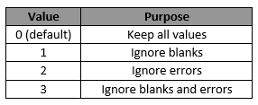
array, ignore, and scan_by_column are the three inputs that the TOROW function accepts. The array or range to be changed is represented by the only mandatory argument, Array. What values TOROW will opportunistically disregard is controlled by the ignore argument. The following are the possibilities for ignore:
3. VALUETOTEXT Function:
Any supplied value is returned as text via the VALUETOTEXT function. It transforms non-text data into text and passes text values in their original form.
- Purpose of the function:
A value is transformed into a text string using the VALUETOTEXT function. Text values typically pass through unaltered by default. But in strict mode, double quotes are used to contain text values (“). No matter the format, VALUETOTEXT will always remove any applied number formatting.
- Syntax:
=VALUETOTEXT(value, [format])
- Arguments:
value- The value that you will text.
format- [optional] The output text’s format.
- 0 or omitted (default): Gives back the readable, concise format.
- 1: returns the strict format with row delimiters and escape characters.
- Explanation a VALUETOTEXT Function with Example:
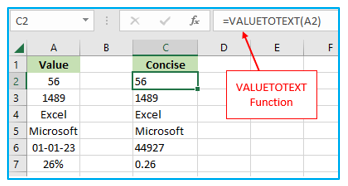
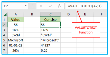
The first value you want to convert to text should be in the same row as a blank cell, such as C2 in this instance. Enter the formula below in that cell, then press the Enter key. To access the remaining results, choose this result cell and drag the AutoFill Handle downward.
=VALUETOTEXT(A2)
You must set the format option to 1 to output data in strict format. Observe this image:
=VALUETOTEXT (A2,1)
- Explanation of output result:
You won’t see double quotes (“) in any of the output examples, and value is always returned as a regular text string in the first formula, see the first screenshot.
When format is set to 1 (strict) in the second illustration, quotations are inserted into the text and shown on the worksheet.
However, as text values in Excel always appear oriented to the left, you will see the output in cells with the General number format applied with the result aligned to the left. If cell A2 has any numerical formatting (such as currency, percentage, etc.), it will be lost after conversion.
4. VSTACK Function:
To produce a larger array, appends arrays vertically and sequentially.
- Purpose of the function:
Vertically stacking arrays are combined into one array using the Excel VSTACK function. The bottom of the previous array is where the next array is added. A single array that fills many spreadsheet cells is the output of VSTACK.
- Syntax:
=VSTACK(array1, [array2], …) (array1, [array2], …)
- Arguments:
array1- The initial range or array to be combined.
array2- The second array or range to merge, if applicable.
- Explanation a VSTACK Function with Example:
Assume you have two tables like these:
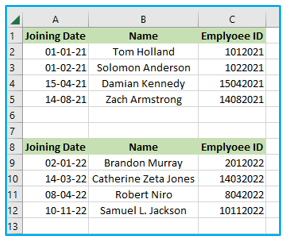
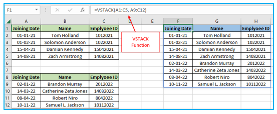
The formula to vertically join two tables is:
=VSTACK(A1:C5, A9:C12)
Various-sized arrays:
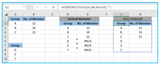
The smaller array will be enlarged to match the size of the larger array when VSTACK is used with arrays of various sizes. In other words, as seen in the example below, the smaller array is “padded” to match the size of the larger array. Cell D2 of the formula reads:
=VSTACK(A1:B4, A8:A10)
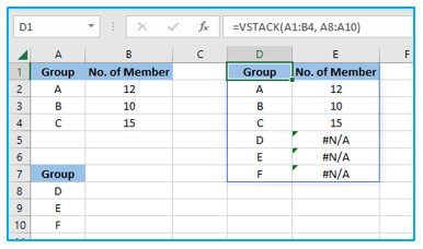
Error code #N/A is shown. Use the IFERROR function to ignore this mistake. The equation in G2 is:
=IFERROR(VSTACK(A1:B4,A8:A10),””)
- Explanation of output result:
In the first illustration, the output of VSTACK is a single array with the same number of rows and columns as the total of all the source arrays.
When two different-sized arrays are used using VSTACK, the smaller array will be enlarged to the size of the larger array. The second example illustrates this by “padding” the smaller array to match the size of the larger array.
The #N/A error will by default appear in the padding-related cells. The IFERROR function is one method for catching these issues.
In the final illustration, an empty string (“”) is used as the error replacement by the IFERROR expression, which results in an empty cell.
5. WRAPCOLS Function:
after a predetermined number of elements, creates a new array by enclosing the row or column of values provided by columns.
- Purpose of the function:
By wrapping values into distinct columns, the Excel WRAPCOLS function creates a two-dimensional array from a one-dimensional array. The wrap count input specifies the length of each column; when the count is reached, WRAPCOLS begins a new column.
- Syntax:
=WRAPCOLS(vector, wrap_count, [pad_with])
- Arguments:
vector- The range or array to wrap.
wrap_count- Each column’s maximum values.
pad_with- [optional] Value to be applied to blank spaces.
- Explanation a WRAPCOLS Function with Example:
Your original data’s structure may make it appropriate to be reorganized into columns (WRAPCOLS). The maximum number of values that can be entered into each column is determined by the wrap count option.
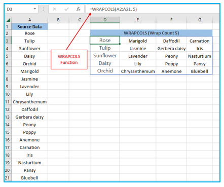
Use this formula, for instance, to convert the range A2:A21 into a 2D array where each column can hold up to 5 values:
=WRAPCOLS(A2:A21, 5)
The illustration below depicts how this appears:
- Explanation of output result:
The maximum number of values for each column is represented by the wrap_count. A new column is started by WRAPCOLS Function once the count has been achieved. You can see how this operates in the screenshot above. The wrap_count in the D3 formula is 5.
6. WRAPROWS Function:
After a predetermined number of elements, creates a new array by wrapping the row or column of values provided by rows.
- Purpose of the function:
By splitting data into distinct rows, the Excel WRAPROWS function expands a one-dimensional array into a two-dimensional array. The wrap count input specifies the length of each row; when the count is reached, a new row is created by WRAPROWS.
- Syntax:
=WRAPROWS(vector, wrap_count, [pad_with])
- Arguments:
vector- The range or array to wrap.
wrap_count- Maximum values per row.
pad_with- [optional] Value to be applied to blank spaces.
- Explanation a WRAPROWS Function with Example:
You might decide that rearranging your original data into rows is appropriate depending on how it was originally structured (WRAPROWS). The maximum number of values that can be contained in each column and row is set by the wrap count option.
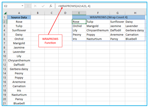
Use this formula, for instance, to create a 2D array from the range A2 to A21 where each row has a maximum of 4 values:
=WRAPROWS(A2:A21, 4)
The illustration below depicts how this appears:
- Explanation of output result:
The maximum number of values for each row is represented by the wrap_count. A new row is started by WRAPROWS Function once the count has been achieved. You can see how this operates in the screenshot above. The wrap_count in the E2 formula is 4.
Please visit for ready-to-use dashboards:
