Logical Functions in Excel are the cornerstone of sophisticated data analysis and decision-making processes, enabling you to perform complex checks and automate responses based on specific criteria. This comprehensive guide explores the array of logical operators and functions available in Excel, such as IF, AND, OR, and NOT, illustrating how they can be combined and nested to create powerful formulas. Whether you’re aiming to streamline your workflow, analyze large datasets, or implement dynamic decision trees, understanding how to effectively use logical functions in Excel will unlock new levels of efficiency and insight in your data management tasks.
In spreadsheets, logical operations excel are used to determine whether a scenario is true or false. You will then be able to take one or another based on the results of that test.
The information displayed, various computations made, or further tests run can all be done using Microsoft excel logical functions.
This Tutorial Covers:
- Excel AND Function
- Syntax of the excel AND operator
- Arguments of the AND operator in excel
- How to Use AND Function in Excel (With example)
- Limitations of AND Function
- Excel FALSE Function
- Syntax of the FALSE Function
- Arguments of the FALSE Function
- How to Use the False Function in Excel (With example)
- Things to Remember About FALSE Function in Excel
- Excel IFS Function
- Syntax of the IFS Function
- Arguments of the IFS Function
- How to Use the IFS Function in Excel (With example)
- Excel IFERROR Function
- Syntax of the IFERROR Function
- Arguments of the IFERROR Function
- How to Use the IFERROR Function in Excel (With example)
- The IFERROR function in Excel has five items you should be aware of
- Excel NOT Function
- Syntax of the NOT Function
- Arguments of the NOT Function
- How to Use the NOT Function in Excel (With example)
- Excel OR Function
- Syntax of the OR Function
- Arguments of the OR Function
- How to Use the OR Function in Excel (With example)
- Excel TRUE Function
- Syntax of the TRUE Function
- Arguments of the TRUE Function
- How to Use the TRUE Function in Excel? (With example)
- Things to Remember About TRUE Function in Excel
1. AND Function in Excel – Logical Functions in Excel
Excel’s AND Function is a logical operation that checks several conditions and returns “true” or “false” based on whether or not they are satisfied. “=AND(logical1,[logical2]…),” where “logical1” is the first condition to be evaluated, is the formula for the AND function.
- Syntax of the AND Function:
This is how the syntax is presented:
=AND(

- Arguments of the AND Function:
These essential arguments are accepted by the function:
- The first condition or logical value to be assessed is “logical 1”.
- The second criterion or logical value to be assessed is “logical 2”.
Arguments “logical 1” and “logical 2” are both necessary but optional.
- How to Use AND Function in Excel?
There are three subjects and five students in an exam. To pass the exam, a student must pass all three subjects. The student fails if he/she fails in any of the three subjects.
The performance of the students in different subjects is given in the following table. We are required to determine who passes.
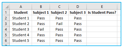
Step 1: As seen below, use the formula in column E2 and press enter key on your keyboard and the fill the other cell.
=AND(B2=”Pass”, C2=”Pass”, D2=”Pass”)
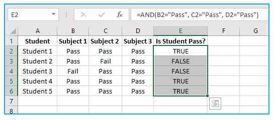
Explanation:
Student 1, Student 4 and Student 5 have passed all the subjects. Since all the logical conditions for these three students are met, the AND function gives the output “true.”
The rest of the students were unable to pass all three subjects. If any of the subjects is not passed, the AND function returns “false.”
- Limitations of AND Function:
The limitations are as follows:
- The AND function can examine approximately to 255 arguments starting with Excel 2007 as long as the formula’s length doesn’t go over 8,162 characters.
- With a formula length of no more than 1,024 characters, the AND function in Excel 2003 and earlier versions can test up to 30 arguments.
- If logical conditions are given as text or if none of the parameters evaluate to a logical value, the AND function returns “#VALUE! error”.
- In the event that all of the supplied parameters are empty cells, the AND function produces “#VALUE! error.”
2. Excel FALSE Function:
When used in a blank cell, the Excel FALSE function is a logical function that outputs “FALSE.” The TRUE function in Excel is similar to this function in that it does not accept any arguments. Instead, it is combined with other conditional functions, such as the IF function, to determine whether or not the condition is met and return “FALSE” as a value.
- Syntax of the FALSE Function:
This is how the syntax is presented:
=FALSE

- Arguments of the FALSE Function:
The FALSE Function on Excel requires no arguments.
Excel will recognize the term “FALSE” entered straight into any cell or formula as the logical value “FALSE.”
- How to Use the False Function in Excel? (With example):
The Boolean value FALSE is what the FALSE function returns. In other words, the following three IF function-based formulas are similar in terms of functionality:
=IF(A1>80,”OK”,FALSE())
=IF(A1>80,”OK”,FALSE)
=IF(A1>80,”OK”)
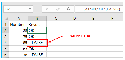
If the value in A1 is not larger than 80, then all three formulas produce FALSE.
Working with the logical values “OK” and “FALSE,” the IF function. We should note that the IF function will automatically return “FALSE” as seen above if we do not specify the “value if false” parameter.
- Things to Remember About FALSE Function in Excel:
- “FALSE” is the logical value that the function returns.
- The FALSE and FALSE () are both the same.
- The value of the FALSE function is 0.
- TRUE and FALSE are the only two logical values. The polar opposite of false is TRUE.
- There is no argument necessary for the function.
3. Excel IFS Function – Nested IF Functions
Nested IF functions, meaning one IF function inside of another, allow you to test multiple criteria and increases the number of possible outcomes. An Excel built-in function known as the IFS function returns results based on one or more true or false conditions.
Syntax of the IFS Function:
This is how the syntax is presented:
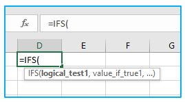
=IFS(
- Arguments of the IFS Function:
The conditions are referred to as logical test1, logical test2, …, which can verify things like:
- If a number is greater than another number >
- If a number is smaller than another number <
- If a number or text is equal to something =
Each condition is connected with a return value.
- How to Use the IFS Function in Excel?
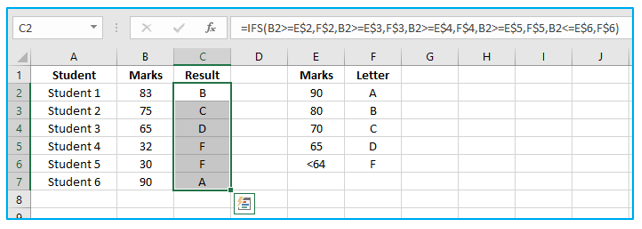
Step 1: Choose cell C2 and enter the formula as shown below and press enter key on your keyboard.
=IFS(B2>=E$2,F$2,B2>=E$3,F$3,B2>=E$4,F$4,B2>=E$5,F$5,B2<=E$6,F$6)

Step 2: Fill the rest cells by autofill handle. The result looks like below.
4. Excel IFERROR Function:
Excel’s IFERROR function is made to detect and handle calculation and formula errors. IFERROR, in further detail, verifies a formula and, if it evaluates to an error, returns a different value you specify; otherwise, it returns the formula’s outcome.
- Syntax of the IFERROR Function:
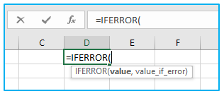
IFERROR is a function in Excel with the following syntax:
IFERROR(value, value_if_error)
- Arguments of the IFERROR Function:
These essential arguments are accepted by the function:
- Value (mandatory)- What to check for mistakes. It could be a formula, expression, value, or cell reference.
- Value_if_error (mandatory) – what to return in the event of an error. It could be a blank cell, text message, numeric value, formula, or calculation.
- How to Use the IFERROR Function in Excel? (With example):
For instance, if one of the columns contains empty cells, zeros, or text, you can receive a variety of problems while dividing two columns of integers.
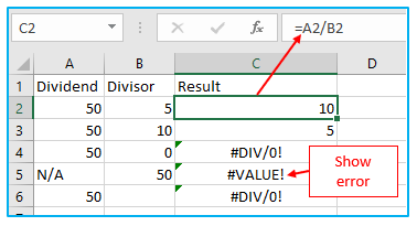
IFERROR, then blank:
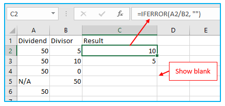
Use the IFERROR function to identify and manage errors as you see fit to avoid that from occurring.
To return a blank cell if an error is encountered, pass the value if error option an empty string (“):
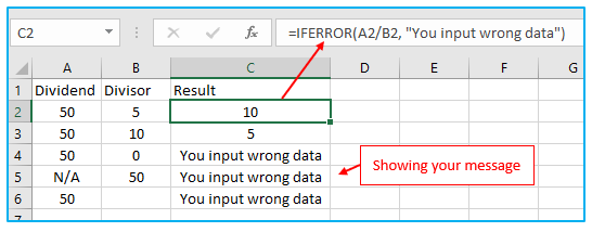
=IFERROR(A2/B2, “”)
IFERROR, then display a message:
In addition of Excel’s default error notation, you can indeed insert your customized message:
=IFERROR(A2/B2, “You input wrong data”)
- The IFERROR function in Excel has five items you should be aware of:
- Including #DIV/0!, #N/A, #NAME?, #NULL!, #NUM!, #REF!, and #VALUE!, all error kinds are supported by Excel’s IFERROR function.
- IFERROR can substitute errors with your personalized text message, a number, a date, a logical value, the outcome of another formula, or an empty string, depending on the values of the value if error parameter (blank cell).
- Blank cells are regarded as empty strings (“‘) but not as errors if the value argument is a blank cell.
- IFERROR was first introduced in Excel 2007 and is now present in Excel 2010, Excel 2013, Excel 2016, Excel 2019, and Excel 365.
Use the ISERROR function along with IF, as demonstrated in this example, to detect problems in Excel 2003 and older versions.
5. Using the NOT Function in Excel
The Excel NOT function is a logical operation referred to as the negation operation. It negates the value that a function or another logical function returned. The logic, which might be a formula or a logical value, is the only argument for this built-in Excel function.
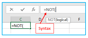
- Syntax of the NOT Function:
NOT is a function in Excel with the following syntax:
=NOT(
- Arguments of the NOT Function:
These essential arguments are accepted by the function:
Logical: It makes sense that all other values are considered “True,” while the number 0 is regarded as “False.” An expression is said to be logical if it calculates the TRUE or FALSE and returns TRUE or FALSE depending on whether the expression is TRUE or FALSE.
- How to Use the NOT Function in Excel? (With example):
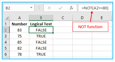
Here, the NOT function is used to run a logical test on the provided set of numbers. Here, we’ll determine which value exceeds or is equal to 80.
The table has two columns: the first is a column for numbers, and the second is a column for logical tests where the NOT function is applied.
As a result, it will output the opposite value. It will output FALSE if the value is greater than or equal to 80 and TRUE if the value is less than or equal to 80.
6. Using the OR Function
Excel’s OR function is a logical operation that determines if at least one of several conditions is true. If only one of the conditions is true, the value does not fail the test.
- Syntax of the OR Function:
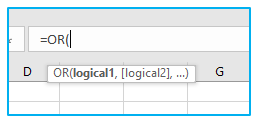
The OR function’s syntax, or format, is as follows:
=OR(logical1, [logical2],…)
- Arguments of the OR Function:
logical1 – The first condition or logical value to evaluate.
logical2 – [optional] The second prerequisite or logical value to assess.
There is only one argument needed. However, it is likely that you will have at least two if you’re employing an OR function.
- How to Use the OR Function in Excel?
Using the OR function in a real-world scenario is demonstrated here. The employer wants to reward everyone who puts in overtime and has perfect attendance with bonuses. The employee would be eligible for that incentive if any of these two conditions was met.
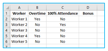
Two statements are necessary to determine the rows that fit one or both requirements. Both the first and second statements would imply that the value in cell D2 equates to the word “Yes.” The following would be the OR formula:
=OR(B2=”Yes”, C2=”Yes”)
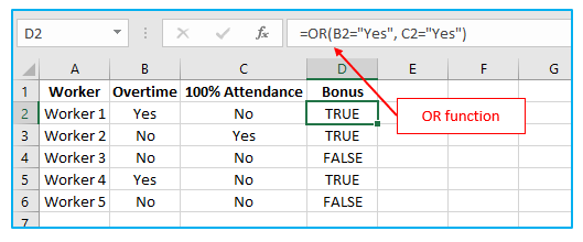
If both claims are accurate, the outcome TRUE is shown. The result TRUE is shown if at least one of the statements is accurate.
Excel returns a value of FALSE if neither claim is accurate.
7. Excel TRUE Function Tutorial
The Excel function TRUE is a logical function that works without any input. This function returns TRUE as its output because it is a TRUE function. Other conditional functions, like the IF function, employ this formula to determine whether the output is “TRUE” if the condition is satisfied or “FALSE” if it is not.
- Syntax of the TRUE Function:
The TRUE function’s syntax, or format, is as follows:
=TRUE()

- Arguments of the TRUE Function:
The Excel formula for TRUE has no parameters or arguments.
- Learn How to Use the TRUE Function in Excel?
We’ll now examine how to combine an IF function with a TRUE function. We’re looking to see if the values below are larger than 80 (evaluate to true).
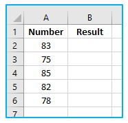
Procedure of using TRUE function in Excel:
Step 1: We will apply the following formula for this in cell B2:
=IF(A2>80,TRUE())
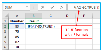
Step 2: After pressing the enter key on your keyboard, fill the rest cells by autofill handle.
The result looks like below.
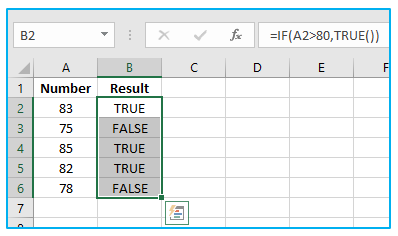
If the condition is satisfied, it will return TRUE; otherwise, it will return FALSE.
- Things to Remember About TRUE Function in Excel:
- With other functions, a mainly TRUE function is utilized.
- The outcome of the TRUE function without the parentheses is TRUE ().
- In a mathematical calculation, TRUE is consistently equal to 1 and FALSE to 0.
- When we perform computations on TRUE and FALSE, the outcome will occasionally be like follows:
TRUE + FALSE = 1
TRUE + TRUE = 2
- Using the TRUE formula directly will cause Excel to produce the logical value TRUE if we want the result to be TRUE.
For Example: IF(250>0, TRUE()) , IF(150<200, TRUE)
- Boolean values TRUE or FALSE are automatically returned as output by logical expressions.
- With TRUE and False functions, we can also perform numerical calculations like:
TRUE() * 25 = 25
FALSE()* 40 = 0
- The TRUE function enables us to determine whether a given condition is true.
Application of Excel Logical Functions or Logic Functions
Here are some uses of logical functions in Excel:
- Conditional Data Analysis and Decision Making:
- Utilize the IF function to perform different actions based on whether a condition is true or false, such as assigning a pass/fail status based on test scores or calculating bonuses based on sales targets.
- Complex Criteria Testing:
- Combine the AND, OR, and NOT functions with IF to test multiple conditions simultaneously, enabling sophisticated decision-making processes, like determining eligibility based on several criteria.
- Data Validation and Error Checking:
- Implement logical functions to validate data entries, ensuring they meet certain criteria or flagging inconsistencies, like identifying orders that fall outside of typical quantity ranges.
- Automating Task Status or Project Milestones:
- Use logical functions to automatically update the status of tasks or project milestones based on completion of certain criteria, facilitating project management and tracking.
- Creating Dynamic Formulas:
- Build dynamic formulas that adjust calculations or outputs based on changing data or user inputs, enhancing the adaptability and intelligence of your financial models or analytical tools.
- Sorting and Filtering Data:
- Employ logical functions within sorting and filtering operations to organize and view data that meets specific conditions, making data analysis more targeted and efficient.
Logical functions are a fundamental aspect of Excel, offering the flexibility and power needed to perform a wide range of data analysis and decision-making tasks efficiently.
You may be interested:
