Index Match Formula in Excel is a powerful tool for performing advanced data lookup and retrieval tasks. By combining the INDEX and MATCH functions, users can efficiently search for and retrieve data from a specified range or array based on specific criteria. Unlike VLOOKUP or HLOOKUP, the Index Match Formula in Excel offers greater flexibility and accuracy, especially when dealing with large datasets or non-contiguous data. Whether you’re working with complex spreadsheets, databases, or financial models, mastering the Index Match Formula in Excel can significantly enhance your productivity and efficiency. With its ability to handle dynamic ranges, multiple criteria, and exact or approximate matches, this formula is a preferred choice for Excel users seeking precise and reliable data retrieval solutions. Incorporating the Index Match Formula in Excel into your repertoire empowers you to tackle a wide range of data manipulation tasks with ease and precision.
- What is INDEX MATCH in Excel?
- How to use INDEX in Excel?
- How to use MATCH in Excel?
- How to use INDEX and MATCH together in Excel?
- The INDEX syntax Function.
- The match syntax function.
- Tips and tricks for index match.
- Some common errors of index match.
- 4 Reasons to use index match as an alternative to VLOOKUP.
1. What is INDEX MATCH in Excel?
In Excel, the INDEX MATCH function can be used to match values from one column to another while searching for information in a table. INDEX MATCH stands out from his VLOOKUP due to its increased adaptability and flexibility. It can address more complex scenarios where VLOOKUP is not functioning properly. The INDEX MATCH Formula combines the INDEX and MATCH functions in Excel. A table’s cell value is returned by =INDEX() depending on the column and row numbers. The position of a cell within a row or column is returned by =MATCH(). The two formulas can retrieve a cell’s value from a table using both vertical and horizontal criteria.
2. How to use INDEX function in Excel?
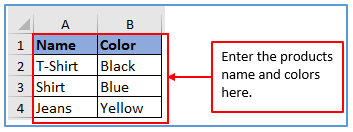
Step 1: Create a data table with the names of some products and colors as shown below.
You can see the name of the products along with colors are written down here.
Step 2: Add a column in D1 and D2 to get the index function value there.
Added the column here.

Step 3: Here you can refer to the formula of the index. Refer to A1:B4 which is the total area of the table then input the row number(3) regarding which you want to find after that refer the column number(2)
So, the formula will be: =INDEX(A1:B4,3,2). Used the formula here.

Step 4: After entering the formula press enter to get the value.
Here is the result below.

3. How to use Match function in Excel?
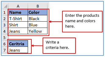
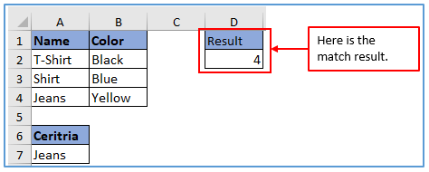
Step 1: Take some product name and their color as the information and create a data table with that information and write the criteria you want to get the result of here is the criteria is Jeans.
Placed the information here.
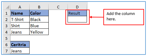
Step 2: Now, add another column in D1 and D2 to get the value there.
The column has been added here.
Step 3: Here you can refer to the formula of the match. Refer to A8 which is the criteria of the table then input the A1:A4 name column which is find the criteria value after that refer to the exact number(0)
The formula will be: =MATCH(A7,A1:A4,0). Applied the formula here.
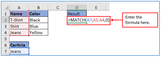
Step 4: In the end, hit enter to get the value.
The result is outlined below.
4. How to use INDEX and MATCH together?
In the world of spreadsheets, index and match together refers to a powerful combination of two functions in software like Microsoft Excel: INDEX and MATCH. Used individually, they serve different purposes, but when combined, they become a versatile tools for performing advanced lookups and data retrieval.
Step 1: Create a data table with the information below.
Placed the information here.

Step 2: Now, add a column in F1,F2 and G1,G2 and choose a month and a name to get the output there as shown below.
You can see the column has been added here.

Step 3: Here you can refer table from Jan to Mar (B2:D5) and put the match function and select the criteria G1 then refer A2:A5 which matches the criteria value after that use 0 for the exact match and lastly refer column number(2). For this the formula will be: =INDEX(B2:D5,MATCH(G1,A2:A5,0),2)
Added the formula here.

Step 4: Press enter to get the value.
Here is the result below.

5. The INDEX syntax Function.
=INDEX(array, row_num, [column_num])
array need: The range or array of cells remains unchanged.
When an array has only one row or column, the appropriate argument for this row’s or columns’ num should be left unspecified.
If a particular array has multiple rows and multiple columns, and only row_num or columns_nm is used, INDEX returns an array of the entire number of rows or column in the array.
row_num: Required. If column_num does not exist. Choose the array column from which you wish to return a value. Columns_num must be specified if row is not included.
column_num: Optional. Determine the column in the array to return true. If Column_num is omitted, Row_num is required.
6. The MATCH syntax Function.
=MATCH(lookup_value, lookup_array, [match_type])
lookup_value (Required): Identifiers to match in the search_array field. In a phone book, the search value for identifying someone’s number is their name; however, what about their phone number? How does this work? Lookup_value can be either a numeric, textual, or logical value, and preferably referred to as the value itself, such as arbitrary numbers or data.
lookup_array (Required): Range of cells to be searched.
match_type (Optional): Number -1, 0, or 1. The matching of lookup_value and lookout_array in Excel is governed by the match_type argument’s semantics. It can be used as a starting point for the argument is 1.
7. Tips and tricks for index match.
Here are a few tricks you can use to make the most out of your time.
- Use named ranges:By creating tables and named ranges of lookup values, it is possible to bypass manual input of cell references. Formulas are made easier to read and maintain thanks to this.
- Use INDEX MATCH in arrays:If you want to search for multiple values at once, curly brace syntax can be used by INDEX MATCH on arrays. For instance, INDEX(range to search, MATCH (value 0), INDERX (2range) To filter all possible matches, we use the following sequence: >INDEX (1referenced range); REF.
- Sort your tables:Tables can be sorted in any order, but INDEX MATCH recommends using ascending or descending orders to optimize search results and improve readability.
Byfollowingtheseguidelines,youcanenhanceyourExcelskillswithINDEXMATCH.
8. Some common errors of index match.
Like other Excel functions, using INDEX MATCH can result in errors. These errors are frequently occurring due to the absence of the search value in the table. The following items can be considered errors:
- #N/A error: Checking for errors in spelling involves checking if the search value is correct or has extra spaces. The IFERROR function can be employed to rectify this error and exhibit a personalized message.
- #REF error: Takes place if the search or comparison range is moved away or shifted. Correct the error by ensuring that any updated cell references in your formulas are correct.
- #VALUE error:Named ranges are an alternative to prevent accidental deletions. Inputs that contain the wrong data type are responsible for this error. ConfirmthattheinputdatatypeisaccurateandusetheVALUEfunctiontoperform
It is advisable to verify your input and ensure that the formulas are accurate before using them, as a general rule.By using the Evaluate Formula feature in Excel, you can step by yourself and gain insight into how your formula is evaluated.
9. 4 Reasons to use index match as an alternative to VLOOKUP.
- Right to left lookup: Search from right to left: As experienced users know, VLOOKUP does not allow you to look to the left. That is, the search value must always be in the leftmost column of the table. You can easily search links with INDEX MATCH!
- Safely insert or delete columns: Because the VLOOKUP syntax requires you to specify the index number of the column you want to retrieve data from, the VLOOKUP expression will break or produce incorrect results if new columns are removed from or added to the lookup table.It may be done.Of course, adding or removing columns will change the index number. INDEX MATCH specifies a range of columns to return, not an index number. This allows you to insert and delete as many columns as you want without worrying about updating all the associated expressions.
- There is no limit to the size of the search value: When using the VLOOKUP function, the total length of the search criteria cannot exceed 255 characters. If it exceeds 255 characters, #VALUE! will be displayed error. Therefore, if your dataset contains long strings, INDEX MATCH is the only valid solution.
- Processing speed will be faster: If your table is relatively small, there will be little difference in Excel performance. However, if your worksheet contains hundreds or thousands of rows and therefore hundreds or thousands of formulas, Excel only needs to search and return columns rather than the entire table array. MATCH INDEX works much faster than VLOOKUP.
The impact of VLOOKUP on Excel performance can be especially noticeable if your workbook contains complex array formulas such as VLOOKUP or SUM. The important thing is that you need to call the VLOOKUP function separately to check each value in the array. The more values your array contains and the more array formulas you have in your workbook, the slower Excel will perform.
Application of Index Match Formula in Excel
- Complex Lookups: Use INDEX MATCH for complex lookups, especially when data is not sorted or structured conventionally, allowing you to retrieve information from any column, surpassing VLOOKUP’s left-to-right limitation.
- Two-Way Lookups: Perform two-dimensional lookups by matching both rows and columns, ideal for searching through matrices or tables to find specific data points, such as prices in different regions.
- Dynamic Column References: Apply INDEX MATCH to dynamically refer to columns in your formulas, making your spreadsheets more adaptable when adding or removing columns, without needing to update formula references manually.
- Handling Large Datasets: Utilize INDEX MATCH for efficient data retrieval in large datasets, as it tends to be faster and less memory-intensive than VLOOKUP, especially when dealing with thousands of rows.
- Data Validation and Error Handling: Enhance data validation and reduce errors by using INDEX MATCH. It provides more precise control over lookup values and return results, helping to avoid common errors associated with data mismatches.
- Creating Flexible Dashboards and Reports: Incorporate INDEX MATCH in dashboards and reports for flexible data retrieval, allowing you to easily update and maintain dynamic reports without redoing the entire setup for new data ranges or criteria.
You may be interested:
