Hyperlink in Excel concludes your journey towards creating interactive, user-friendly spreadsheets that not only guide users efficiently but also connect them to a wealth of information with just a click. This powerful feature transforms your static sheets into dynamic maps of data, where every link is a pathway to deeper insights and resources. Embrace the full potential of hyperlinks in Excel to navigate through your data landscape with ease, making your spreadsheets not just a collection of numbers, but a network of knowledge, accessible and organized at your fingertips.
The article demonstrates three distinct ways of Excel hyperlink. You’ll learn how to add, edit, and delete hyperlinks from your worksheets, as well as how to fix broken links.
On the Internet, hyperlinks are frequently used to move between websites. You may build these linkages with ease in your Excel workbooks as well. You may also add a hyperlink to open a new Excel file, send an email, or navigate to a different cell, page, or workbook, or if you want to link a website to your text. In-depth instructions on how to accomplish this in Excel 2016, 2013, 2010, and prior versions are provided in this lesson.
This Tutorial Covers:
- What is hyperlink in Excel
- How to insert a hyperlink in Excel
- Insert links by using the Hyperlink feature
- Create links by using the HYPERLINK function
- Insert hyperlink in Excel programmatically
- How to edit hyperlinks in Excel
- How to remove hyperlinks in Excel
- Tips for using hyperlinks in Excel
- Select a cell without opening a link
- Extract URLs from hyperlinks
- Convert a worksheet object into a clickable hyperlink
- Excel hyperlinks not working
- Stop Automatic Hyperlinks in Excel
1. What is Hyperlink in Excel?
A hyperlink in Excel is a reference to a particular place, file, or web page that the user can access by clicking the link.
You can build hyperlinks in Microsoft Excel for a variety of uses, such as:
- Navigating to a certain place within the active worksheet
- Accessing a specific location within a document, such as a sheet in an Excel file or a bookmark in a Word document, or opening another document.
- Accessing a website through the Internet or an intranet
- Making a new Excel document
- Delivering an email to a predetermined address
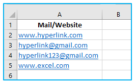
Excel hyperlinks are simple to spot since they typically appear as blue-underlined text, like in the screenshot below.
2. How to Insert Hyperlink in Excel?
The same activity can frequently be completed with Microsoft Excel in several different methods, and this is also true for adding hyperlinks. You can use any of the following methods to insert hyperlink in Excel:
- Hyperlink Insert dialog box.
- HYPERLINK function.
- VBA code.
- Insert links by using the Hyperlink feature:
The Insert Hyperlink dialog, which has three different methods to be reached, is the most popular method for immediately inserting a hyperlink into a cell.
Method 1: From the “Insert” tab
The procedure of inserting links by using hyperlink feature:
Step 1: Choose the cell where you want to insert the hyperlink in excel.
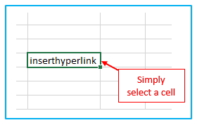
Step 2: Depending on the version of Excel you are using, select the “Hyperlink” or “Link” button under the “Links” group on the “Insert” tab.

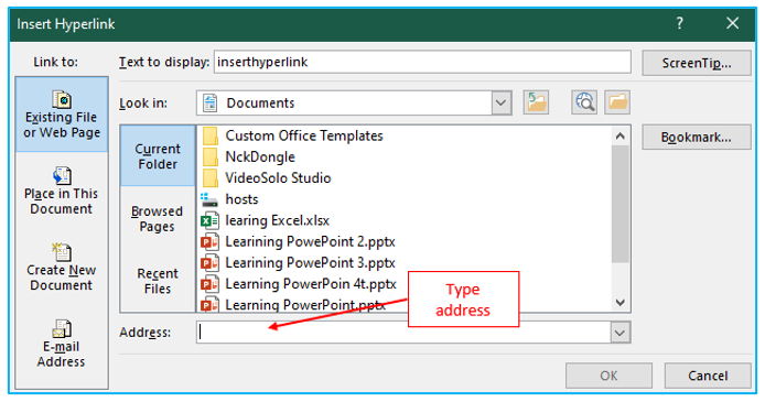
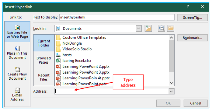
Step 3: After that, the “Insert Hyperlink” dialog box appeared. Then, type the address as your desired in the “Address” box. Then click OK.
The result looks like below.

Method 2: From the “Context” menu
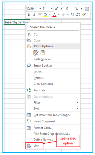
Step 1: Select “Hyperlink” (Link in more recent versions) from the context menu by right-clicking the cell.
Step 2: Depending on the version of Excel you are using, select the “Hyperlink” or “Link” button under the “Links” group on the “Insert” tab.

Step 3: After that, the “Insert Hyperlink” dialog box appeared. Then type the address as your desired in “Address” box. Then click OK.
The result looks like below.

Method 3: Using shortcut key
Step 1: Simply choose the cell where you want to add the link.
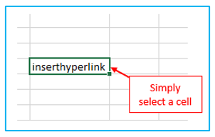
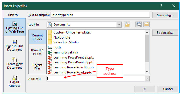
Step 2: Press Ctrl + K on your keyboard. After that, “Insert Hyperlink” dialog box appeared. Then type address as your desired in “Address” box. Then click OK.
After that, the result looks like below.

Now choose from one of the following examples, depending on the type of link you wish to make:
- Hyperlink to another document
- Hyperlink to web-page (URL)
- Hyperlink to a sheet or cell in the currently open workbook
- Hyperlink to a new workbook
- Hyperlink to an email address
Create the hyperlink to another document:
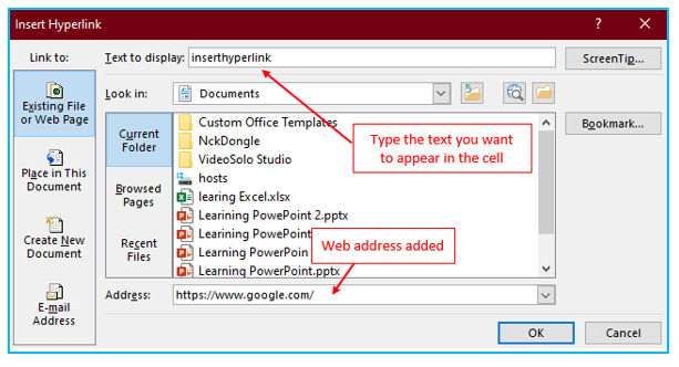
Open the “Insert Hyperlink” window and follow the steps listed below to insert a hyperlink to another document, such as a different Word, Excel, or PowerPoint presentation.
Step 1: Click the “Existing File or Web Page” link under “Link to:” in the left-hand panel.
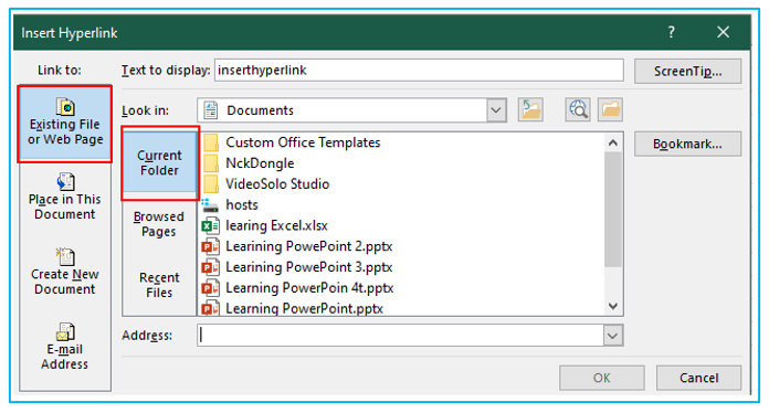
Step 2: Navigate to the target file’s location in the “Look in” list, then pick the file.
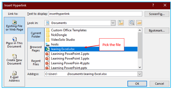
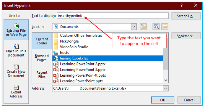
Step 3: Type the text you want to appear in the cell in the Text to show box (“inserthyperlink” in this example). Then click OK.
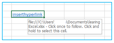
The hyperlink is added to the cell you’ve chosen and appears exactly as you’ve set it up:
Add a hyperlink to a web address (URL):
Open the “Insert Hyperlink” dialog and follow these steps if you want to create a link to a website:
Step 1: Choose “Existing File or Web Page” under “Link to:”.
If you want to link a specific web page, click the “Browse the Web” button, navigate to the desired website, and then return to Excel without closing the browser.
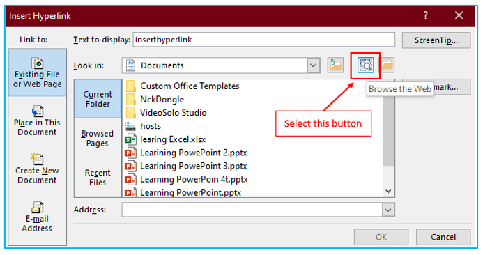
Step 2: Excel will automatically insert the website address and hyperlink text for you to view. If necessary, input a screen tip, edit the wording to how you want it to appear, and then click OK to add the hyperlink.
As an alternative, you can simply paste the URL of the web page in the Address box after copying it and opening the Insert Hyperlink dialog.
Hyperlink to a sheet or cell in the currently open workbook:
Click the “Place in this Document” icon to insert a link to a specific sheet in the open workbook. Choose the target worksheet from Cell Reference, then click OK.
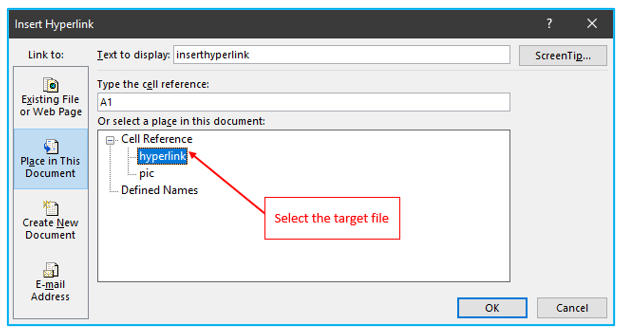
Enter the cell reference in the “Type in the cell reference box” to generate an Excel hyperlink to that specific cell.
Select a named range beneath the “Defined Names” node to link to it.
Insert a hyperlink to open a new Excel workbook:
You can build a hyperlink to a fresh Excel file in addition to existing files. Open the “Insert Hyperlink” dialog and follow these steps to insert a hyperlink to open a new Excel workbook.
Step 1: Under “Link to:”, click the “Create New Document” icon, outlined in Red below.
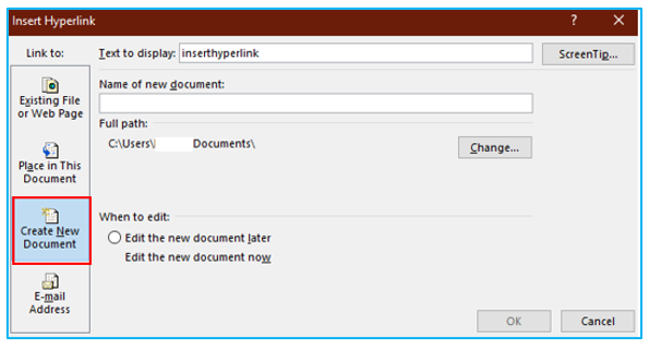
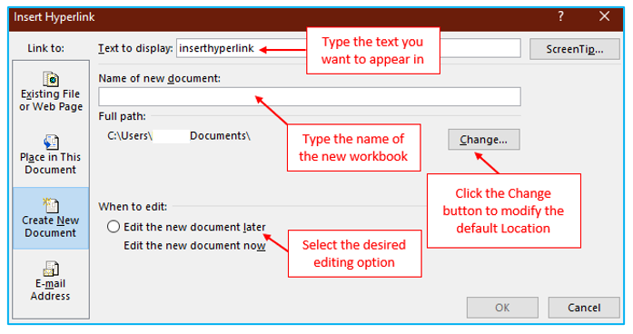
Step 2:
- Type the link text you want to appear in the cell in the “Text to display” box.
- Enter the name of the new workbook in the “Name of new document” box.
- Select the location where the newly produced file will be saved under “Full path”. Click the “Change” button to modify the default position.
- Select the desired editing option under “When to edit”.
Complete the required steps and then select OK.
Create hyperlink to an email address:
You can send an email right from your worksheet using the Excel Hyperlink feature in addition to linking to various documents. Open the “Insert Hyperlink” dialog and take the following actions to get it done:
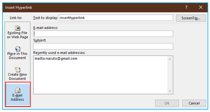
Step 1: Choose the “E-mail Address” icon under “Link to:”.
Step 2:
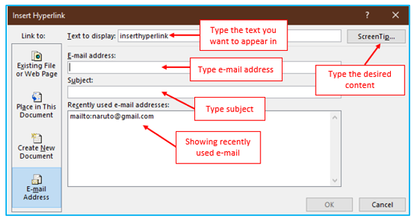
- Enter the recipient’s email address, or several addresses separated by semicolons, in the “E-mail Address” box.
- Optionally, fill out the “Subject” box with the message’s subject. Please be aware that some email applications and browsers might not recognize the subject line.
- Type the required link text into the “Text to display” box.
- Alternatively, select the “ScreenTip…” button and type the desired content (the screen tip will be displayed when you hover over the hyperlink with the mouse).
Complete the required steps and then select OK.
Tip: Using the email address directly in a cell is the quickest approach to create a hyperlink to a specific e-mail address. Excel will instantly turn it into a clickable hyperlink as you press the Enter key.
- Create links by using the HYPERLINK function:
How to use the HYPERLINK function to create links
The HYPERLINK function can be used to insert hyperlinks in Excel if you are one of those Excel experts who use formulae to complete the majority of jobs. When you want to add, update, or remove numerous links at once, it is especially helpful.
The HYPERLINK function has the following syntax:
HYPERLINK(link_location, [friendly_name])
Where:
- The path to the destination document or web page is indicated by “Link location.”
- The link text to be displayed in a cell is “Friendly name.”
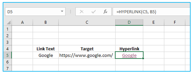
The simplest Excel Hyperlink formula is shown below, where the friendly name is in column B and the link location is in column C:
=HYPERLINK(C5, B5)
The end result can resemble something like this:
- How to use VBA to add a hyperlink to an Excel document
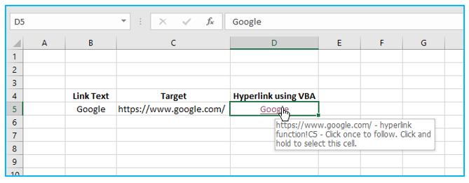
You can automate hyperlink creation in your worksheets by using the following short VBA code:
Public Sub AddHyperlink()
Sheets(“hyperlink function”).Hyperlinks.Add Anchor:=Sheets(“hyperlink function”).Range(“D5″), Address:=”https://www.google.com/”, SubAddress:=”hyperlink function!C5″, TextToDisplay:=”Google”
End Sub
Where:
Sheets: The name of the sheet where the link needs to be placed (hyperlink function in this example).
Range: the cell in which the connection needs to be placed (D5 in this example).
SubAddress: the final destination of the link, or in this case, the hyperlink function!C5.
TextToDisplay – text that will be shown in a cell (“Google” in this example).
Given the information above, our macro will cause the active workbook’s “hyperlink function” to add a hyperlink with the name “Google” in cell D5. You will be directed to cell C5 on the hyperlink feature in the same workbook by clicking the link.
3. How to edit Hyperlink in Excel?
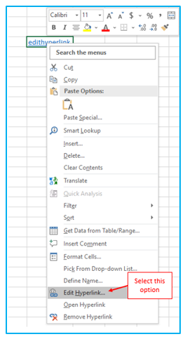
Step 1: Use a dialog identical to the one you used to insert the hyperlink if you need to update it. To do this, either use the context menu by selecting Edit Hyperlink… from a cell’s right-click menu, the shortcut key Crtl+K, or the Hyperlink button on the ribbon.
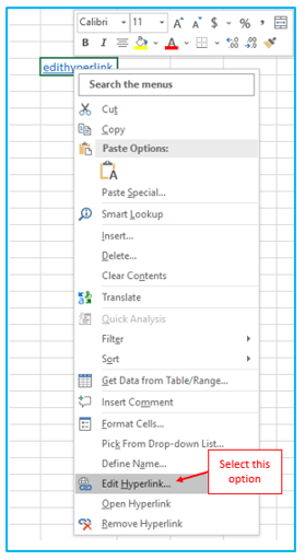
Step 2: Any action you take will cause the Edit Hyperlink dialog box to appear. You click OK after making the desired adjustments to the link wording, link location, or both.
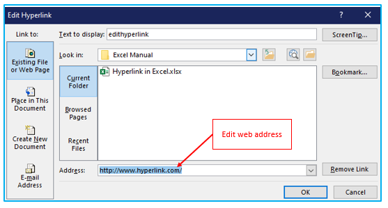
Select the cell holding the Hyperlink formula and adjust its arguments if you want to edit a formula-driven hyperlink. The method for selecting a cell without going to the hyperlink location is described in the following advice.
4. How to remove Hyperlink in Excel?
The procedure of removing hyperlinks in Excel:
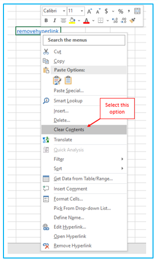
Step 1: In Excel, eliminating hyperlinks requires two clicks. Simply choose Remove Hyperlink from the context menu when you right-click a link.
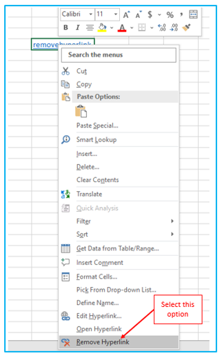
This keeps the link text in a cell but deletes the clickable hyperlink.
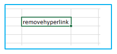
Right-click the cell and select Clear Contents to remove the link text as well.
5. Tips for using Hyperlink in Excel:
You may want to learn a few practical tips to use links most effectively now that you are aware of how to add, edit, and remove hyperlinks in Excel.
- Select a cell without opening a link:
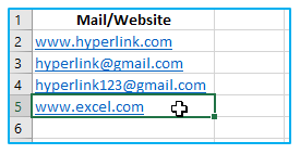
By default, clicking a cell that has a hyperlink opens the target document or web page, which is the link destination. Click the cell, hold down the mouse button until the pointer changes to an Excel selection cursor (a cross), and then release the button to choose a cell without navigating to the link position.
Move the mouse pointer over the whitespace and click the cell as soon as it turns into a cross. If a hyperlink only takes up a portion of a cell (i.e. if your cell is broader than the link’s text), move the mouse pointer over the whitespace and do the following:
- Extract URLs from hyperlinks:
Both manually and programmatically are viable options for removing a URL from an Excel hyperlink.
Extract a URL from a hyperlink manually in Excel:
Following these straightforward procedures will enable you to easily extract the destinations of a small number of hyperlinks:
Step 1: Choose the cell that has the hyperlink in it. After that, open the Edit Hyperlink dialog by pressing Ctrl + K, or right-click and click “Edit hyperlink”
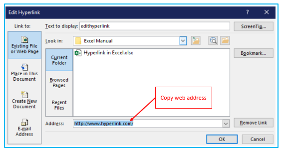
Step 2: Select the URL in the Address area and click Ctrl + C to copy it. To close the Edit Hyperlink dialog box, press Esc or click OK. Insert the copied URL into any available cell. Done!
By using VBA, extract several URLs:
Extraction of each URL manually would be a waste of time if your Excel worksheets contain a large number of hyperlinks. By automatically removing addresses from all of the hyperlinks on the current sheet, the following macro can expedite the process:
Sub ExtractHL()
Dim HL As Hyperlink
Dim OverwriteAll As Boolean
OverwriteAll = False
For Each HL In ActiveSheet.Hyperlinks
If Not OverwriteAll Then
If HL.Range.Offset(0, 1).Value <> “” Then
If MsgBox(“One or more of the target cells is not empty. Do you want to overwrite all cells?”, vbOKCancel, “Target cells are not empty”) = vbCancel Then
Exit For
Else
OverwriteAll = True
End If
End If
End If
HL.Range.Offset(0, 1).Value = HL.Address
Next
End Sub
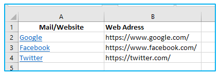
The screenshot below demonstrates how the VBA code extracts URLs from a column of hyperlinks and inserts the information into adjacent cells.
- Convert a worksheet object into a clickable hyperlink:
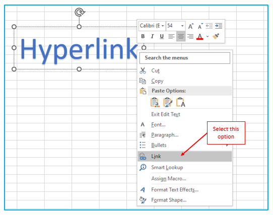
Many worksheet elements, like as charts, photos, text boxes, and shapes, can be made into clickable hyperlinks in addition to text in a cell. Simply right-click an item (in the screenshot below, it’s a WordArt object), select “Link” and insert or add the link as instructed above.
6. Excel Hyperlinks not working:
The following troubleshooting steps will assist you in identifying and resolving any issues with hyperlink functionality in your worksheets.
Reference isn’t valid:
Symptoms: Excel displays an error message that reads “Reference isn’t valid” when a user clicks a hyperlink.
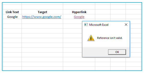
Solution: The name of the sheet is used as the link target when you establish a hyperlink to another sheet. The hyperlink won’t work if you subsequently rename the worksheet since Excel won’t be able to find the target. You can either adjust the hyperlink to point to the renamed sheet or change the sheet’s name back to the original name to remedy this.
You will need to enter the new path to the file if you built a hyperlink to another file and subsequently moved it.
The hyperlink is just an ordinary text string:
Symptoms: Web addresses (URLs) that are written, copied, or imported into your worksheet do not automatically become clickable hyperlinks, nor do they receive the standard blue underlining styling. Or, links may appear to be functional but do nothing when you click on them.
Solution: To edit the cell, double-click it or hit F2 to open the edit mode, then press Space when you reach the end of the URL. A text string can become a clickable hyperlink in Excel. Check the format of your cells if there are a lot of these links. Links inserted in cells using the General format can occasionally cause problems. Try setting the cell format to Text in this instance.
After reopening a worksheet, hyperlinks were inactive:
Symptoms: Up until you saved and opened the workbook again, your Excel hyperlinks were working properly. They are all now gray and out of a job.
Solution: First, make sure the link destination has not changed, meaning the target document has not been moved or renamed. If that isn’t the case, you can think about disabling a setting that makes Excel verify hyperlinks each time the workbook is saved. According to accounts, Excel occasionally removes legitimate hyperlinks (for example, links to files stored in your local network may be disabled because of some temporary problems with your server.) Follow these procedures to disable the option:
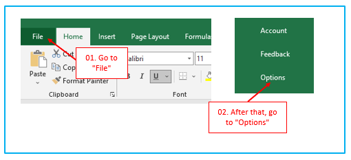
Step 1: When using Excel 2010, 2013, 2016, or 2019, click “File” from the ribbon and then select “Options.” Excel 2007 users should select “Excel Options” from the “Office” menu.
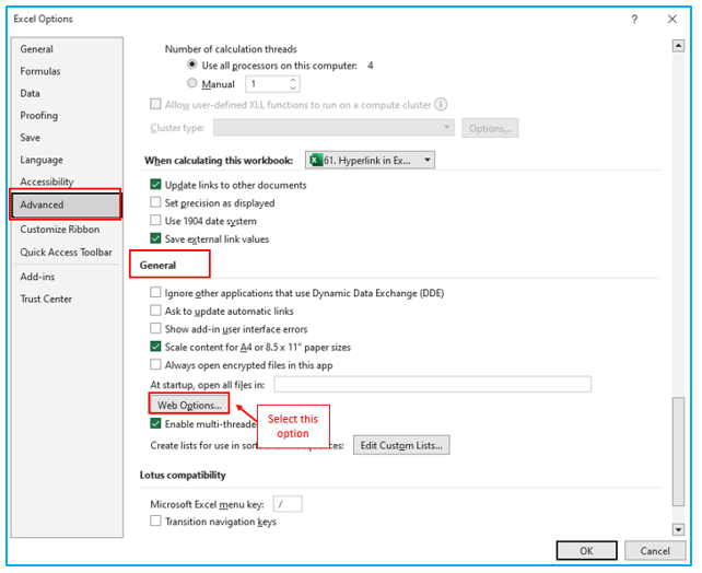
Step 2: Choose “Advanced” from the left-hand panel. Click “Web Options” under “General” by scrolling down.
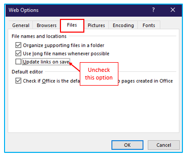
Step 3: Select the “Files” tab in the “Web Options” dialog, uncheck the “Update links on save” box, and then click OK. This how to disable this option.
7. Stop Automatic Hyperlink in Excel:
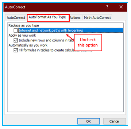
You can disable the hyperlinking feature if you don’t want links generated when you type a website address.
How to turn the hyperlink option off is shown below.
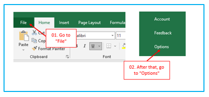
Step 1: When using Excel 2010, 2013, 2016, or 2019, click “File” from the ribbon and then select “Options.” Excel 2007 users should select “Excel Options” from the “Office” menu.
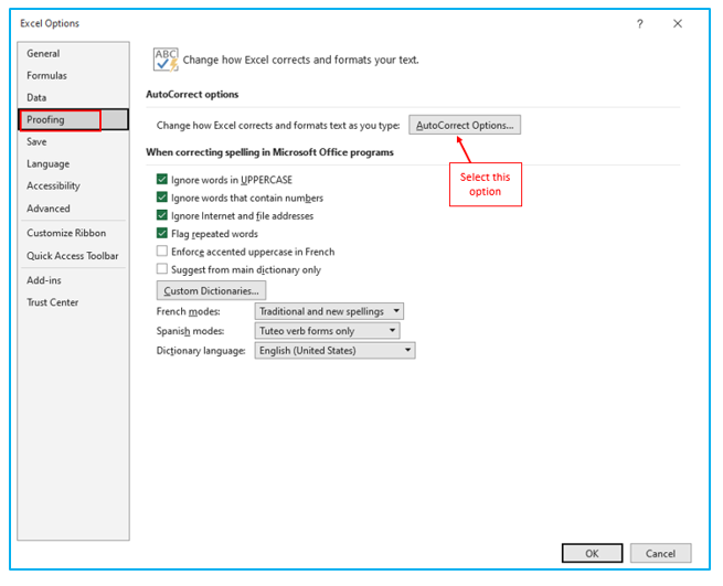
Step 2: Click the “AutoCorrect Options…” option under the “Proofing” category.
Step 3: The “AutoFormat As You Type” tab’s “Internet and network paths with hyperlinks” option should be unchecked. For the dialog boxes to close, click OK twice.
You may be interested:
