XLOOKUP in Excel revolutionizes the way users search and retrieve data within spreadsheets, offering unmatched flexibility and efficiency. This dynamic function allows users to search horizontally or vertically, find exact matches or approximate matches, and retrieve corresponding values effortlessly. Whether you’re navigating large datasets, creating interactive dashboards, or performing complex data analysis, XLOOKUP in Excel streamlines the process with its intuitive syntax and powerful capabilities. Say goodbye to cumbersome VLOOKUP and HLOOKUP functions and embrace the future of Excel functionality with XLOOKUP. With XLOOKUP in Excel, users can navigate through data with ease, making informed decisions faster than ever before.
This Content Covers:
- What is XLOOKUP?
- XLOOKUP Function Syntax, Purpose, and Arguments
- How to Fetch a Lookup Value using XLOOKUP?
- How to Look-up and Fetch an Entire Record using XLOOKUP?
- How to do a Two-way Look-up using XLOOKUP?
- Error Handling using XLOOKUP.
- How to use XLOOKUP Function to Look-up in Multiple Ranges?
- How to Find Tax Rate/Commission Rate using XLOOKUP?
- How to do Conditional Lookup using XLOOKUP and Other Functions in Excel?
- XLOOKUP with MAX and MIN Functions
- XLOOKUP with COUNTIF Function
1. What is XLOOKUP?
The XLOOKUP is a built-in function in Microsoft Excel which is only available in Office 365. This is an upgraded version of VLOOKUP or HLOOKUP. With the help of this function, you can identify a value in a horizontal or vertical dataset and obtain the value that corresponds to it in some other columns or rows.
2. XLOOKUP Function Syntax, Purpose, and Arguments
Syntax: =XLOOKUP(lookup_value, lookup_array, return_array, [if_not_found], [match_mode], [search_mode])
Purpose: The purpose of this function is to lookup values in range or array
Arguments: There are three compulsory and three optional arguments in this function,
lookup_value- The value to look for.
lookup_array- The array or range in which we are looking for the value.
return_array- The array or range to return.
[if_not_found] (optional)- If the lookup value cannot be found, this value will be returned. An #N/A error will be returned if you don’t specify this argument.
[match_mode] (optional)- Here you can specify the type of match you want,
0 = exact match (default), -1 = exact match or next smallest, 1 = exact match or next larger, 2 = wildcard match.
[search_mode] (optional)- Here you specify how the XLOOKUP function should search the lookup_array,
1 = search from first (default), -1 = search from last, 2 = binary search ascending, -2 = binary search descending.
3. How to Fetch a Lookup Value using XLOOKUP?
Suppose we have this dataset, and we want to get the sales amount for Fiona (the lookup value)
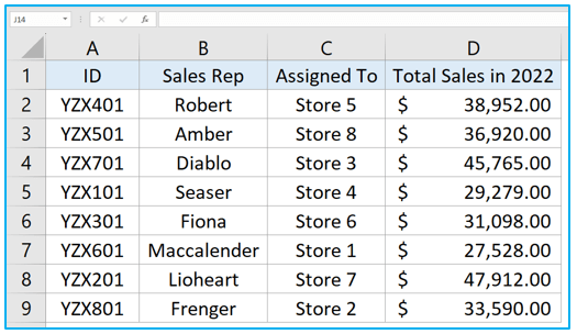
Step 1: Type or copy the lookup value in another cell.
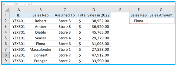
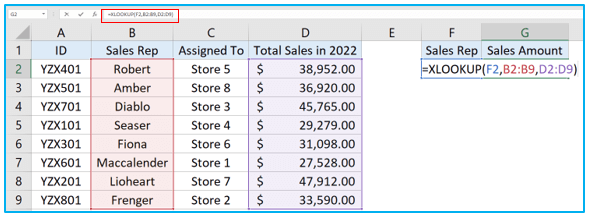
Step 2: Insert the following formula in the cell where you would like to get the result.
=XLOOKUP(F2,B2:B9,D2:D9)
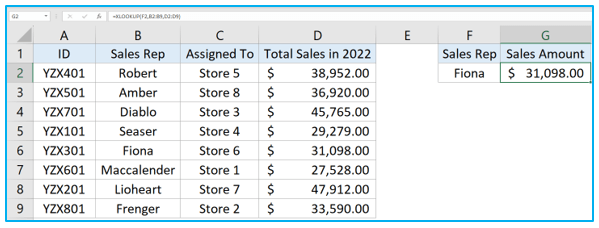
Step 3: Press Enter key to get the result.
4. How to Look-up and Fetch an Entire Record using XLOOKUP?
Suppose you want to get the entire record for the sales-rep whose id is YZX701.

Step 1: Select the cell where you want the result to be displayed and insert the below given formula inside the cell.
=XLOOKUP(F2,A2:A9,B2:D9)

Step 2: Hit the Enter button to get the corresponding result.

5. How to do a Two-way Look-up using XLOOKUP?
Suppose we want to know which shop/store the sales rep whose id no is YZX701 is assigned to. We can do this by using the first method that we have seen. But here we will see how we can use the two-way look-up to get the result and what benefit it gives us.
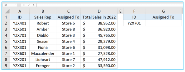
Step 1: Insert this formula in G2.
=XLOOKUP(G1,B1:D1,XLOOKUP(F2,A2:A9,B2:D9))

Step 2: Hit Enter to get the result.
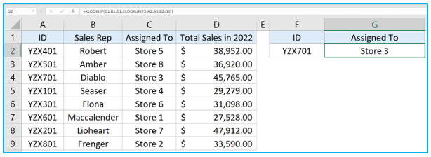
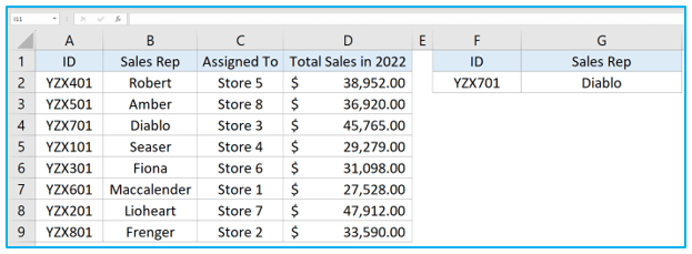
Step 3: The benefit of using two-way lookup is that if you change the title of G1, the result will change too. Suppose you want to know the name of this sales rep, all you have to do is change the title of G1 from Assigned To, to Sales Rep.
6. Error Handling using XLOOKUP.
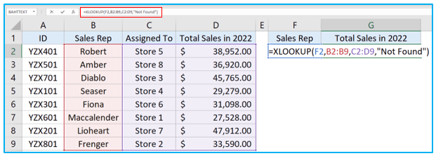
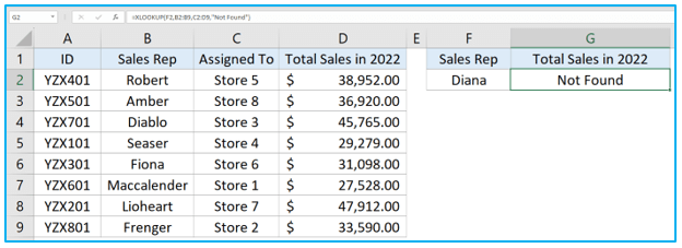
Here we were searching for the total sales amount for the sales rep Diana which resulted in #N/A error. This happened because there is no sales rep named Diana on our list. While working with large datasets, we might find this error quite often. With the help of XLOOKUP function we can set our custom error text that the function should return if a value can’t be found.
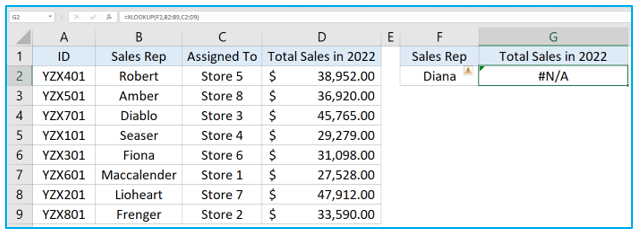
Step 1: Type your custom error text inside the formula.
Step 2: Hit the Enter key.
7. How to use XLOOKUP Function to Look-up in Multiple Ranges?
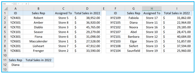
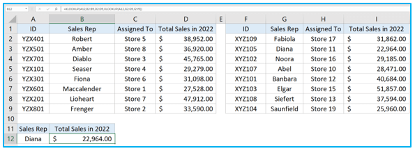
In this worksheet we have two data tables instead of one and we don’t know in which one the sales rep Diana is. Now we have to look for the sales amount for Diana by looking up both of these ranges together by using a Nested LOOKUP Formula.
Step 1: Insert this nested XLOOKUP formula in B12.
=XLOOKUP(A12,B2:B9,D2:D9,XLOOKUP(A12,G2:G9,I2:I9))
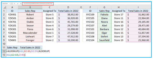
Step 2: Press Enter key to get the result.
8. How to Find Tax Rate/Commission Rate using XLOOKUP?
Suppose we have this datasheet here and on the right-side table we have the sales amount for which the commission will be given and the commission rate.
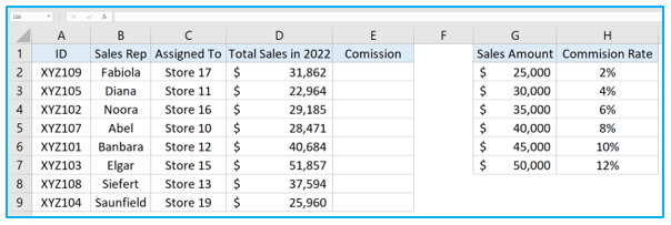
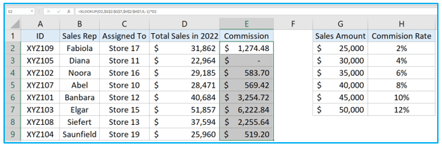
Step 1: Select cell E2 and insert the following formula in this cell. Press Enter key to get the Commission.
=XLOOKUP(D2,$G$2:$G$7,$H$2:$H$7,0,-1)*D2

Step 2: Now drag the fill-handle down to apply the formula on the other cells of this column. The formula here takes the data in D2 as the lookup value and looks through the lookup table on the right. Here we have used -1 as the fifth argument inside the formula which means that it will look for an exact match, and if it doesn’t find one, it will return the value just smaller than the lookup value. In the commission column cell E3 is empty because the total sales amount of D3 (lookup value) is lower than the lowest sales amount for which the commission will be given. So, this person will not get any commission.
9. How to do Conditional Lookup using XLOOKUP and Other Functions in Excel?
9.1 XLOOKUP with MAX and MIN Functions
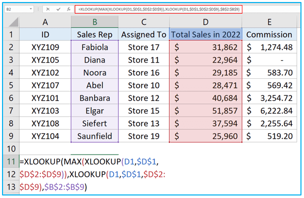
Suppose we have this datasheet, and we want to know who the best and worst sellers are based on their total sales.
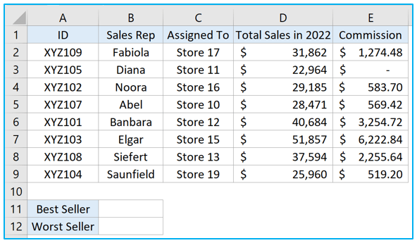
Step 1: Insert the below given formula inside cell B11.
=XLOOKUP(MAX(XLOOKUP(D1,$D$1,$D$2:$D$9)),XLOOKUP(D1,$D$1,$D$2:$D$9),$B$2:$B$9)
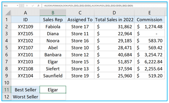
Step 2: Press Enter to get the best seller. The formula has returned Elgar as the best seller. From the Total Sales column we can see that he has the highest total sales, which is $51857.
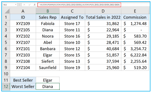
Step 3: Here we used MIN function with XLOOKUP function to get the worst seller which is Diana who has the lowest total sales of $22964.
=XLOOKUP(MIN(XLOOKUP(D1,$D$1,$D$2:$D$9)),XLOOKUP(D1,$D$1,$D$2:$D$9),$B$2:$B$9)
9.2 XLOOKUP with COUNTIF Function
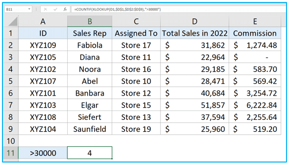
We can use COUNTIF function with XLOOKUP to set a condition in order to know how many sellers have sold more than $30000.
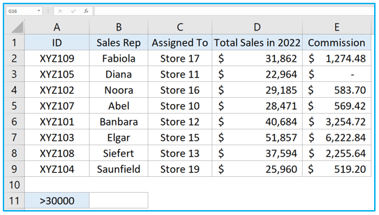
Step 1: Select the cell where you want the result to be displayed and insert this formula.
=COUNTIF(XLOOKUP(D1,$D$1,$D$2:$D$9),”>30000″)
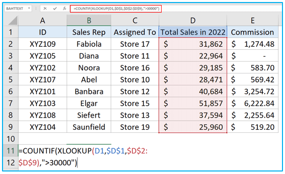
Step 2: Press Enter key to get the result in that cell.
Application of XLOOKUP in Excel
- Dynamic Data Retrieval: Utilize XLOOKUP in Excel to dynamically retrieve data from tables based on specified criteria, simplifying data analysis tasks.
- Vertical and Horizontal Lookup: Perform both vertical and horizontal lookups with XLOOKUP, enabling flexible data retrieval across different orientations within spreadsheets.
- Exact and Approximate Matches: Find exact matches or approximate matches with XLOOKUP, providing versatility in searching for data within Excel tables.
- Handling Errors: XLOOKUP handles errors more efficiently compared to traditional lookup functions, reducing the likelihood of #N/A errors and improving data integrity.
- Replacing VLOOKUP and HLOOKUP: Transition from VLOOKUP and HLOOKUP to XLOOKUP for improved functionality and ease of use, as XLOOKUP combines the features of both.
- Array-Like Behavior: XLOOKUP can return entire columns or rows of data as arrays, enabling more advanced calculations and data manipulation within Excel.
For ready-to-use Dashboard Templates:
