How to use OFFSET formula in Excel?

OFFSET formula in Excel is a powerful tool that allows you to dynamically reference cells based on specified rows and columns. By mastering this formula, you can create flexible ranges, automate data retrieval, and enhance the functionality of your spreadsheets. Whether you’re working with large datasets, building complex reports, or automating calculations, the OFFSET formula in Excel streamlines your workflow and improves efficiency. Incorporating this formula into your daily Excel tasks will help you create dynamic, adaptable solutions that save time and reduce manual errors. Embrace the OFFSET formula in Excel to elevate your data management and analysis capabilities.

What is the OFFSET formula in excel?
How to use offset formula in Excel?
When to use Excel OFFSET in excel?
How to use the Excel OFFSET function in Excel?
- OFFSET and SUM
- OFFSET and AVERAGE / MAX / MIN
- Excel OFFSET formula to sum the last N rows
Notes About the OFFSET Function in Excel.
The OFFSET Limitations
The OFFSET function

1. What is the OFFSET formula in Excel?

The purpose of Excel OFFSET is to provide reference data for each cell or range thereof.

By entering a reference point, the user can determine which direction it moves in.

At a new point in the program, the formula determines which adjacent cells should be returned.

Syntax of OFFSET formula: =OFFSET(Reference, Rows, Cols, [Height], [Width])

A reference is a cell or range of cells that serves as a starting point for a formula.

Rows are the numerical value that represents the number of rows that move up or down from the formula’s starting point.

Columns are the number of columns that move left or right according to the formula.

Height indicates the height of the returned area.

Width indicates the width of the returned range.

2. How to use offset formula in Excel?

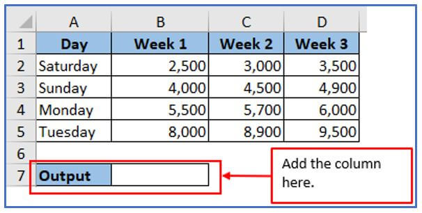
Step 1: Create a data table with the weekly earnings of 3 weeks below.

You can see the week name and earnings are written down here.

Step 2: Add a column in D1 and D2 to get the offset function value there.

Add the column here.

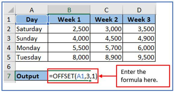
Step 3: Here you can refer to the formula of the OFFSET function. So, the formula will be: =OFFSET(A3,3,1)

Here, A1 is for the column of week name

3 is for the three rows deep in the right column as chosen here.

1 is for selecting week 1.

Use the formula here.

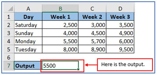
Step 4: After entering the formula press enter to get the value.

This gives us a value of 5,500 three rows deep in the right column, as shown below.

In the example above, the returned range has the same height and width as the reference range, so we omitted the reference.

3. When to use Excel OFFSET in Excel?

In Excel, the OFFSET function can be employed to identify a set of cells that is dynamically defined based on specific criteria or conditions.

The OFFSET function can be used in various scenarios, as demonstrated below.

Dynamic Range: OFFSET allows you to create a dynamic range that automatically adjusts when data is added, deleted, or rearranged within a worksheet. It can be utilized to construct dynamic charts, pivot tables, or data analysis tools.
Scrolling or Sliding Windows: OFFSET allows you to create scrolling or sliding windows of data within a larger data set. The use of OFFSET can enable you to view specific rows or columns within an interactive dashboard or report, which permits you access to data by scrolling.
Conditional Formatting: By using OFFSET, it is possible to apply formatting to a dynamic range of cells under particular circumstances through conditional formatting.
Data Analysis: In data analysis, OFFSET can be applied to tasks that require calculations or extracting subsets of data using changing criteria.
Creating dynamic formulas: With OFFSET, it is possible to generate formulas that refer to different cell ranges dynamically, depending on the conditions. For example, you can use OFFSET to calculate moving averages, running totals, or other time series analysis metrics.

In essence, OFFSET is a versatile feature that can be used to dynamically reference multiple cells in an Excel spreadsheet, regardless of any changing conditions or criteria. Although OFFSET can use resources in large datasets or complex expressions, it is important to use it carefully and consider alternative methods if needed.

4. How to use the Excel OFFSET function in Excel?

4.1 OFFSET and SUM

Step 1: Here are given every month’s bonus in the table. Each month, a new row is added directly above the SUM formula. Of course, this must be included in the total. In essence, it is manually updating the range in the SUM expression each time here. Means, here used the normal SUM formula.

So, place the information first.

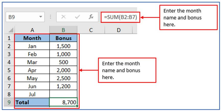
Step 2: Now, add another column in D1 and D2 to apply the OFFSET SUM formula there.

The column has been added here.

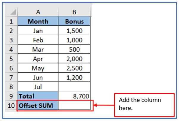
Step 3: Here you want to let the OFFSET expression update it automatically.

Refer to the formula of the match. The formula will be: =SUM(first cell:(OFFSET(cell with total, -1,0) or =SUM(B2:(OFFSET(B9, -1, 0)))

In this case, the B9 is used as a reference for any cell that contains the sum. Row – Cell just above the sum that requires a negative number -1. The column should be set to 0 as not interested in changing the column.

ApplY the formula here.

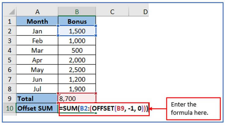
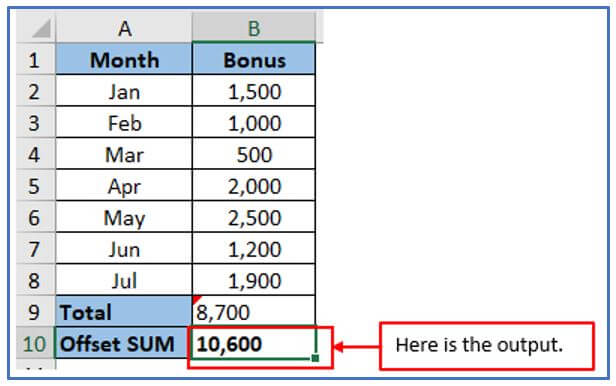
Step 4: In the end, hit enter to get the value. You can see here in Column B10 that, the OFFSET Sum column automatically updates the values after entering the July month bonus amount but the normal total sum amount is the same as before.

The result is outlined below.

4.2 OFFSET and AVERAGE / MAX / MIN

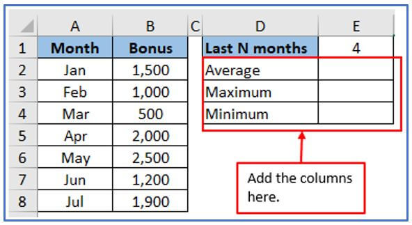
Step 1: Create a data table with the information below.

Placed the information here.

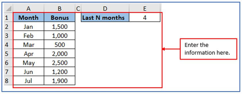
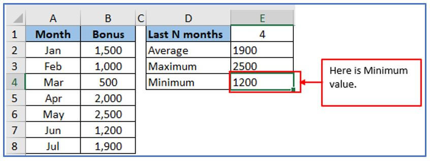
Step 2: Now, add a column from D2:D4 and E2:E4 to get the AVERAGE, MAX ,MIN output there

You can see the column has been added here.

Step 3: Now, use the formula. For Average the formula will be: =AVERAGE(OFFSET(B1,COUNT(B:B)-E1+1,0,E1,1))

Add the formula here.

Step 4: Press enter to get the value.

Here is the Average value.

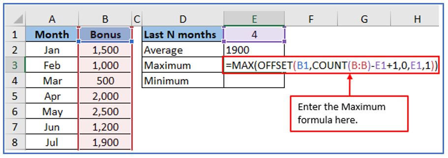
Step 5: Now, use the Maximum formula: =MAX(OFFSET(B1,COUNT(B:B)-E1+1,0,E1,1))

Used the formula here you can see below.

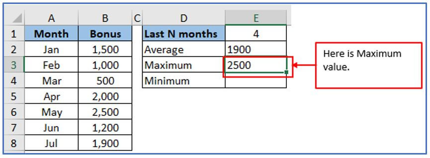
Step 6: Press enter now.

Here is the Maximum Value.

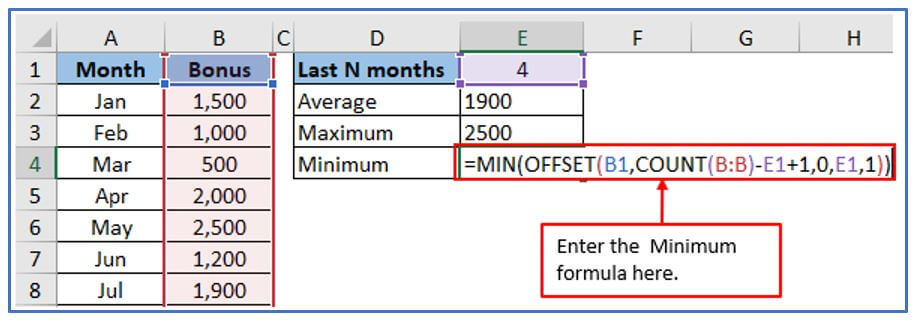
Step 7: Now, use the Minimum formula: =MIN(OFFSET(B1,COUNT(B:B)-E1+1,0,E1,1))

Apply the formula here.

Step 8: Press enter to get the value.

Here is the minimum value is outlined below.

4.3 Excel OFFSET formula to sum the last N rows

Step 1: Suppose you want to know the amount of your bonus over the past N months, rather than the total amount. Here want to the formula that auto-integrates new rows that are inserted into the sheet. For this here is used Count and Counta formula.

Make a table with the month’s name and bonus amount.

Place the numbers here.

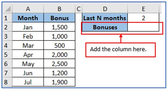
Step 2: Add another column D1 and E1 to get the output there.

You can see below the column has been added here.

Step 3: Here used the COUNT formula. You can use the COUNTA formula as well.

The formula: =SUM(OFFSET(B1,COUNT(B:B)-E1+1,0,E1,1))

=SUM(OFFSET(B1,COUNTA(B:B)-E1,0,E1,1))

Apply the formula here.

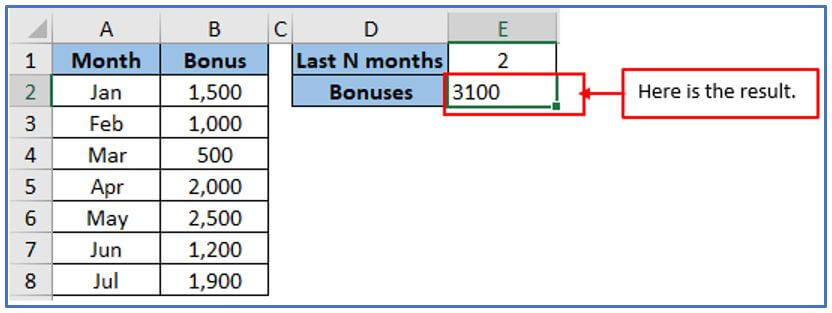
Step 4: After entering the formula press enter button.

The result of the last N rows is shown below.

5. Notes About the OFFSET Function in Excel.

1. The return of cells using OFFSET is limited to a reference.
2. Both row and column can be specified as negative numbers to reverse the normal offset direction. Negative columns are offset to the left and negative rows are offset to the top.
3. The term OFFSET denotes a “volatile function”. Volatile features can slow down larger and more complex workbooks.
4. When not included in height or width, we use the base height and width instead.
5. Functions which anticipate receiving a reference can also utilize OFFSET.
6. According to the documentation in Excel, height and width cannot be negative, but they can be positive.
7. #Reference!Error – Occurs when the range obtained from the requested offset is invalid. For example, it extends beyond the edges of the worksheet.
8. #Value!Error – Occurs if any of the specified row, column, [height], or [width] arguments are non-numeric.

6. The OFFSET function Limitations Limitation

The Excel OFFSET function’s resource-intensive nature, like other volatile functions, poses significant limitations. Excel runs a little longer because the OFFSET formula is recalculated each time the source data changes. This is not a problem for a single expression in a small table. However, if your workbook contains dozens or hundreds of formulas, recalculations in Microsoft Excel can take a significant amount of time.
Excel’s OFFSET formula is difficult to validate. Due to the dynamic nature of the OFFSET function, debugging large formulas can be challenging, especially when dealing with nested DIRECTORIES and SOLVED.

The OFFSET alternative

Excel tables

Excel Spreadsheets So-called “calculated columns” that, when you enter a formula in a cell in an Excel spreadsheet, automatically copy the formula to all other cells in that column, adjusting the formula in each row can be created inside the table. Additionally, formulas that reference data in a table are automatically adjusted to include new rows that you add to the table or exclude rows that you delete. Technically, such formulas operate on columns or rows of tables that are dynamic range in nature. Each table within a workbook has a unique name.

Excel INDEX function

Excel INDEX Function Excel INDEX can also be used to create dynamic range references, although it cannot be used in the same way as OFFSET. In comparison to OFFSET, the INDEX function is nonvolatile and won’t cause Excel to slow down.

Excel INDIRECT function

Creating dynamic ranges from cell values, text, and named interval labels is possible with the INDIRECT function in Excel. The ability to dynamically reference another Excel spreadsheet or workbook is also available.

Application of OFFSET formula in Excel

Dynamic Range Creation: The OFFSET formula in Excel allows you to create dynamic ranges that automatically adjust as data changes.
Data Lookup: Use OFFSET to retrieve values from cells based on relative positions, enhancing data lookup flexibility.
Moving Averages: Calculate moving averages by combining OFFSET with other functions like AVERAGE, adjusting the data range dynamically.
Dynamic Charts: Create charts that automatically update as new data is added by referencing dynamic ranges with the OFFSET formula.
Conditional Data Extraction: Extract specific rows or columns of data based on criteria, making it easy to automate complex data extraction tasks.
Custom Summaries: Build customized summaries or reports that adapt to different data sets, using OFFSET to pull in varying ranges of data.