How to use MID Function in Excel?

In conclusion, the MID function in Excel is a versatile tool that empowers you to work with text data more efficiently. Whether you need to extract specific characters from a cell, split text into meaningful segments, or manipulate text strings to suit your analysis, the MID function is your go-to solution. By understanding its capabilities and applying it strategically, you can streamline your data processing tasks, enhance your spreadsheet skills, and unlock new possibilities in your work. Make the most of Excel’s MID function to gain control over your text data and excel in your data analysis endeavors. MID Function in Excel – your key to text manipulation and precision.

Mid function is a method to find the mid value of any kind of information. For this method, you have to follow the MID function to get the middle number of data.

These content covers:

1. What is the MID Function?
2. Combining MID with other functions.
3. How to use MID in Excel as a worksheet function?
4. How to use Excel MID Function as a VBA function?
5. How to Extract Substrings in Excel with LEFT, RIGHT, MID Functions?

1. What is the MID Function?

The Excel MID function is a text function that may be used to locate strings and return them from any middle area of the spreadsheet. The text or string itself, the start number or position, and the string’s ending position are all used in this formula to extract the result. In simple words, the MID function in Excel extracts a small part of the string from the input string or returns a required number of characters from text or string.

2. Combining MID with other functions.

Quite often, MID is often combined with other Excel text string functions like LEN, TRIM, SUBSTITUTE, LEFT, RIGHT, FIND, and SEARCH to split data or to extract specific elements from text strings. The original text and/or the desired output may be of either fixed or variable length. Those of variable length usually require a bit of creative thinking, so it’s useful to know the type of value returned for each function to determine the combination that will give the result you want. A summary of these functions is shown below.

Function	Syntax	Return value
LEN	LEN(text)	Number of characters
TRIM	TRIM(text)	Text without leading and trailing spaces
LEFT	LEFT(text, [num_chars])	Text – leftmost character(s)
RIGHT	RIGHT (text, [num_chars])	Text – rightmost character(s)

3. How to use MID in Excel as a worksheet function?

To use the MID function in Excel as a worksheet function, follow these steps:

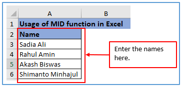
Step 1: Some names have been taken in the example below and the MID function will be found from this name.

Entered the name into the Excel sheet.

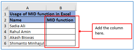
Step 2: Now, add a column in B2:B6 and name it the MID function to get the MID function of those names.

The column has been added here.

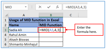
Step 3: Click on the cell where you want to enter the formula. Type the cell reference of the text string from which you want to extract characters. Type a comma (,). Type the starting position of the characters you want to extract. Type a comma (,). Type the number of characters you want to extract. Type ) (closing parenthesis) to complete the formula.

The Formula is: =MID(A3,4,3)

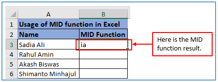
Step 4: Click the enter to get the mid value.

Here you can see the result after clicking enter.

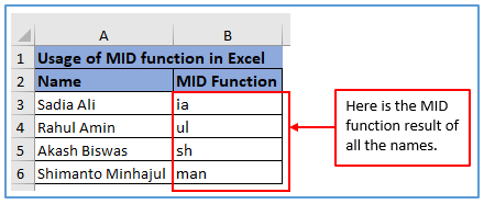
Step 5: Like the way above, use the same formula with changing column number and you will the MID function result of all the names. For Rahul Amin the formula will be: =MID(A4,4,3)

For Akash Biswas, the formula will be: =MID(A5,4,3)

For Shimanto Minhajul, the formula will be: =MID(A6,4,3)

Here is the MID function of all of them.

4. How to use Excel MID Function as a VBA function?

This is the same function as like MID function. But there is a little different at here( VBA ). Here is the example of VBA function in the following below:

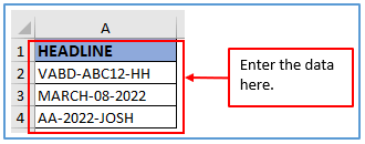
Step 1: First, make some data and put it into Excel as shown in the example.

All the data has been placed here.

Step 2: Now, add a column B1:B4 to get the result there and name MID value.

Column has added.

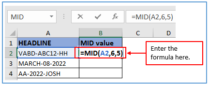
Step 3: Insert the formula. Formula is: =MID(A4,6,5)

Applied the formula in the below image.

Step 4: Now, press Enter.

Here is the answer after applying the formula.

Step 5: Use the same formula for another two Headlines according to the columns and information.

For, MARCH-08-2022 the formula is: =MID(A3,6,5)

For, MARCH-08-2022 the formula is: =MID(A4,6,5)

Here is the output of all.

5. How to Extract Substrings in Excel with LEFT, RIGHT, MID Functions?

The MID function can occasionally be combined with the LEFT and RIGHT operations to distribute values over many cells. As their names imply, LEFT and RIGHT are used to extract the string’s leftmost characters and the rightmost characters, respectively.

In the below example, you can be known with those three substrings in excel ( LEFT, RIGHT, MID).

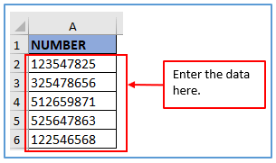
Step 1: Make a data table first.

All the data has been entered here.

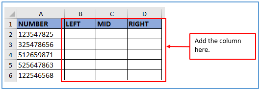
Step 2: Now, add Three  column B1:B6 named it as LEFT column,C1:C6 MID column and D1:D6 as RIGHT column to get the result there .

Three Column has added.

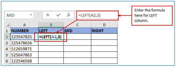
Step 3: Text is the text string to be split. Num_chars is the number of characters in text to return, starting with the leftmost character. If omitted, only the leftmost character is returned.

Insert this formula in LEFT Column: =LEFT(TEXT,NUM_CHARS) or =LEFT(A2,3)

The formula is entered.

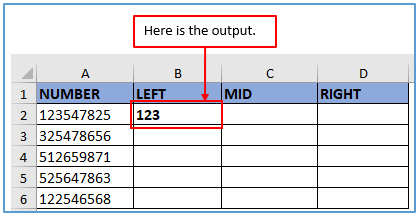
Step 4: After applying the formula click on enter.

Here is the result below:

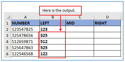
Step 5: Use the same formula for another numbers and change the column number according to the columns or drag down the Excel cursor from B2 and you will get the result of B3:B6 .

Here is the result of LEFT functions.

Step 6: Insert this formula for MID function Column:  =MID(C2,4,3)

Applied the formula here.

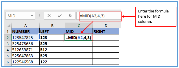
Step 7: After applying the formula click on enter.

Here is the result below:

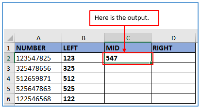
Step 8: Use the same formula for another numbers and change the column number according to the columns or drag down the Excel cursor from C2 and you will get the result of C3:C6 .

Here is the result of MID functions.

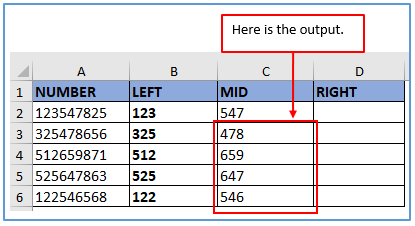
Step 9: : Insert this formula for RIGHT function Column:  =RIGHT(A2,3)

Applied the formula here.

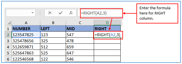
Step 10: After applying the formula click on enter.

Here is the result below:

Step 11: Use the same formula for another numbers and change the column number according to the columns or drag down the Excel cursor from C2 and you will get the result of D3:D6 .

Here is the result of RIGHT functions.

Application of MID Function in Excel

You may be interested:

1. Financial Dashboards
2. Sales Dashboards
3. HR Dashboards
4. Data Visualization Charts