ISNA function in Excel plays a crucial role in ensuring the accuracy and reliability of your data. By checking for #N/A errors, it helps you identify missing or problematic data points, allowing you to make informed decisions based on clean and reliable information. With ISNA function in Excel at your disposal, you can trust that your spreadsheets are free from errors, making your data analysis and reporting processes more efficient and dependable. Don’t overlook the power of this simple yet essential function in Excel, as it can make a significant difference in maintaining data integrity and driving better decision-making.
This content covers:
- What is ISNA Function?
- How to use the ISNA formula in Excel?
- How to use N/A Error with ISNA Function
- How to Use of ISNA with VLOOKUP and IF Functions
- How to Use ISNA Function with NOT Logic
1. What is ISNA Function?
The ISNA function is cataloged as the INFORMATION function in Excel. It is one such function operated to determine whether a cell has errors or not. This only catches one type of error, #N/A, which usually occurs when we try to look for a value in the search range and the value isn’t there. So in the end you get #N/A which summarizes that the value you want is “Not Available” and the ISNA function will detect if the process received #N/A by returning TRUE and FALSE statements.
The ISNA function in Excel is primarily used for error handling and data validation. The most common uses of the ISNA function are:
Check for #N/A errors:
This function allows you to identify cells with #N/A errors and take appropriate actions, such as changing the value to replace the error or change the expression to avoid the error.
Nested formulas:
You can use the ISNA function in conjunction with other functions such as IF and IFERROR to create more complex formulas. For example, you can use this function to test whether a VLOOKUP or INDEX formula returns a #N/A error, and if so, return a specific value or message.
Data Validation:
The ISNA function can be used in data validation rules to ensure that users are entering valid data. For example, you can set up a validation rule that requires users to enter a value other than #N/A in a specific cell or range.
2. How to use the ISNA formula in Excel?
Do make an example like the below picture where have two lists: those who get the results of a particular and those who get marks above 90.
Step 1: First make a list by writing everyone’s name.
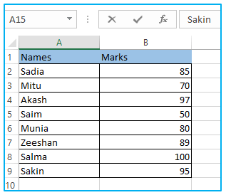
In the picture, you can see there is another table for using formulas and getting the results.
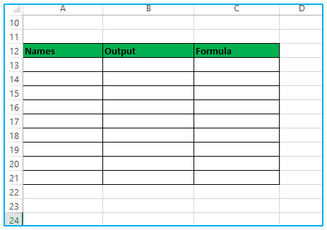
Step 2: Starting in cell A13, enter the name of the student you want to confirm.
You can see below there are three names which you want to work with.

Then Enter the following formula in the adjacent column (B13). =IF(ISNA(VLOOKUP(A13,A2:B9,2,0)),”Student who gets above 90″)
The formula is applied here.
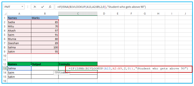
Step 3: Drag the formula down for all cells and you will get Update the formula to display the results.
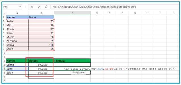
Here is the result after using the formula. If the student is included in the original grade list, the output should be FALSE. This is because the ISNA function returns TRUE or FALSE depending on the condition met.
3. How to use N/A Error with ISNA Function
N/A in a cell is the main function of the ISNA.
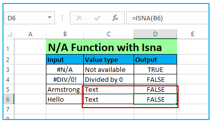
Step 1: First create a dataset like the image.
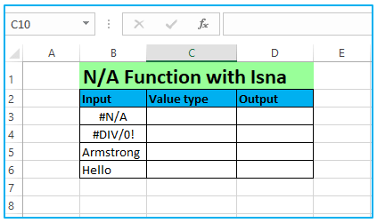
Step 2: In cell B5, you have data #N/A where in the Output column of D we will try to use the ISNA function to see whether the data in cell B3 is available or not.
Using the formula here.
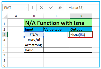
So, the result is True you can see below because the data is not available (#N/A), the function takes back the answer to the question (is the cell’s data available or not?) as it is TRUE. Which means not available.
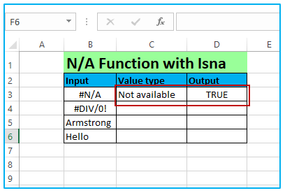
Step 3: You can use the ISNA function to see if the data in cell B6 is available or not. for the second row, you text data, in cell B4. Use the formula =Isna(B4)
You can see the result of B4 is also false because B4 input has a different data type than #N/A and therefore output is also FALSE.
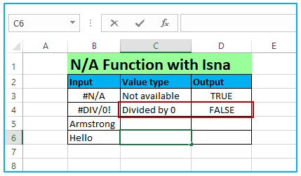
Step 4: Now use the same formula for the rest of the data.
You can see the result is FALSE for B5 an B6 because “Hello” is a text value.
4. How to Use of ISNA with VLOOKUP and IF Functions
It is one of the most admired (and used) look-for functions in Excel.
Step 1: You have to make a dataset.
Here you can see an example with the name of few people,their age and gender.
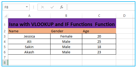
Now you need to set that Name which is shown above as the search value criteria and find the age for it.
Here is entered the search value as NAME and AGE. You will find the age using the VLOOKUP function.
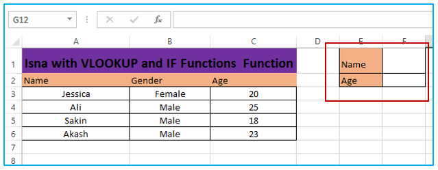
Step 2: The formula: =VLOOKUP(G4,B5:D8,2,0) If E1 has the name SALMA you will find the age of SALMA.
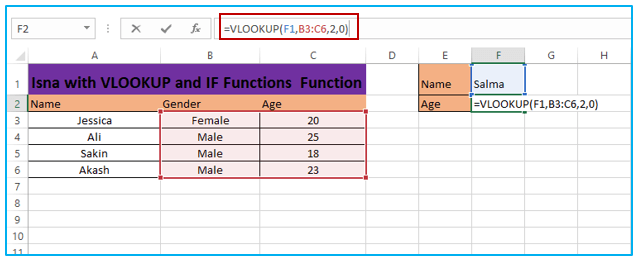
Set a lookup value that is not within the lookup range. Below test it with a name that is not yet listed. Here is Name Salma you can see as the search value.
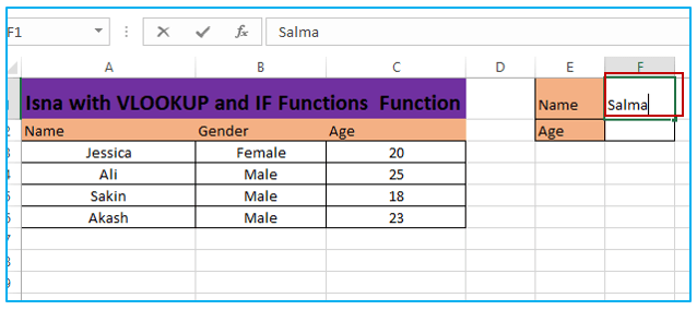
=VLOOKUP(F1,B3:C6,2,0) using the formula here.
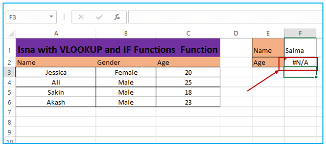
The result is here #N/A because Salma is not available in the table. To solve the problem, we can use the ISNA function along with search functions.
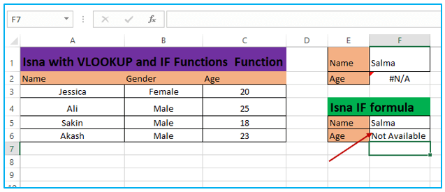
Step 3: Formula for IF function =IF(ISNA(VLOOKUP(E5,A3:C6,2,0)),”Not Available”,VLOOKUP(E5,A3:C6,2,0))
Here is using IF function formula for ISNA.

Here VLOOKUP generates #N/A or not by ISNA. If so, set it to “Unavailable” enabled, otherwise perform a VLOOKUP operation.
Now, as a replacement for of #N/A, you can see “Not available”.
5. How to Use ISNA Function with NOT Logic
Here ISNA function will assist you in implementing NOT LOGIC.
Step 1: First, you have a create a dataset consisting of a number of peoples with corresponding Age and Gender.
It is the dataset of some people with age and gender.
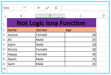
Step 2: If you want to find the number of males who are under age 25 then make a table like below with only male and age.
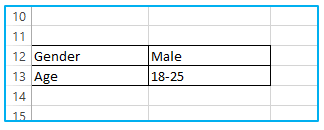
For finding out the male number then the formula will be
=SUMPRODUCT((B3:B9=B12)*ISNA(MATCH(C3:C9,B13,0)))
You have to use a formula like this according to your information and column.
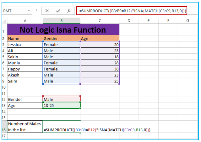
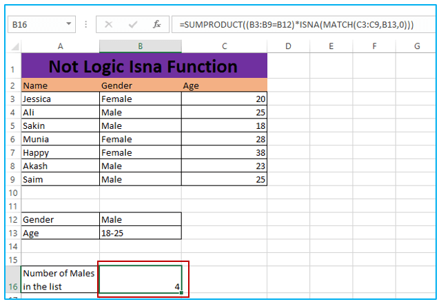
Step 3: After entering the formula press enter. Then you will get the result of, the number of males in the list.
You can see the output that there are 4 males out of 7 people.
Application of ISNA function in Excel
- Error Handling: ISNA is often used in error handling to check if a cell contains the #N/A error value. This helps prevent error messages and allows you to replace the error with a custom message or value.
- Conditional Formatting: You can use ISNA within conditional formatting rules to highlight cells that contain #N/A errors. This makes it easy to identify and correct errors in large datasets.
- Data Validation: When setting up data validation rules, you can use ISNA to ensure that the values entered in a cell are not #N/A errors, thereby improving data accuracy.
- Lookup Functions: ISNA can be combined with lookup functions like VLOOKUP or HLOOKUP to handle cases where the lookup value is not found in the lookup range. It allows you to take specific actions when a match is not found.
- IF Statements: ISNA can be used within IF statements to create conditional logic. For example, you can use it to display a message when a certain condition is met, such as when an #N/A error occurs.
- Array Formulas: ISNA is useful in array formulas where you want to check if any element in an array contains the #N/A error. It returns TRUE if any element is an error, allowing you to perform further actions based on the result.
These are just a few examples of how the ISNA function can be applied in Excel to handle and manipulate data effectively.
You may be interested:
