IFERROR with VLOOKUP in Excel to Replace #N/A Error is a crucial combination for maintaining clean and understandable spreadsheets. This powerful duo ensures that your data lookup tasks are error-free, enhancing the clarity and reliability of your reports. By implementing this strategy, you prevent confusing #N/A errors from cluttering your data analysis, allowing for smoother data interpretation and decision-making processes. Embrace the precision and efficiency of combining IFERROR with VLOOKUP to revolutionize how you handle data discrepancies and improve your overall Excel proficiency.
This Content Covers:
- Definition of IFERROR and VLOOKUP
- What are the reasons for VLOOKUP to return a #N/A Error
- How to use IFERROR with VLOOKUP Replace #N/A Error
3.1 By replacing VLOOKUP #N/A Error with Meaningful Text
3.3 By Sequencing VLOOKUP with IFERROR Function in same sheet
3.3 By Sequencing VLOOKUP with IFERROR Function in different sheets
3.4 Using VLOOKUP with IF and ISERROR
1. Definition of IFERROR and VLOOKUP
VLOOKUP: One of Microsoft Excel’s most helpful and significant features is VLOOKUP. In large data sheets where manual input can be difficult, it is commonly used to search for certain data.
IFERROR: When a formula error is detected, the IFERROR method detects it and delivers a different result or formula. When there is an error, we can use the IFERROR method to either replace the error message with a meaningful text we wish to display or leave it blank.
2. What are the reasons for VLOOKUP to return a #N/A Error
There are multiple reasons for VLOOKUP to return a #N/A error.
- #N/A error may occur if the lookup value contains a single, double, or leading space.
- If any component, data, or value is not found in the formula or if it doesn’t exist.
- Spelling errors can also cause VLOOKUP to return a #N/A Error.
3. How to use IFERROR with VLOOKUP to Replace #N/A Error
In this tutorial today we will show you what are the ways you can use IFERROR with VLOOKUP to replace the #N/A error in your datasheet.
3.1 By replacing VLOOKUP #N/A Error with Meaningful Text

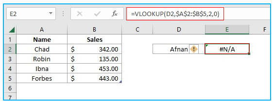
Suppose you have this datasheet and the VLOOKUP formula in Excel you used returned a #N/A error because the value which is put in the formula D2 is not present in the data sheet. Now if you want to replace the error with meaningful text, follow the steps below.
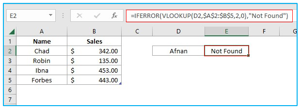
Step 1: Select the cell which shows the #N/A error and change the formula to apply IFERROR and insert a meaningful text at the end of it as shown below.
=IFERROR(VLOOKUP(D2,$A$2:$B$5,2,0),”Not Found”)

3.2 By Sequencing VLOOKUP with IFERROR Function in the same sheet

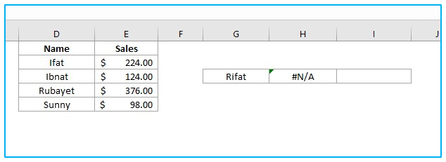
Suppose you have a data table that is fragmented into one sheet or multiple sheets and you want to know a particular value using the VLOOKUP. For example, the picture above has two tables, and you want to know the sales data of Rubayet. To do that that you have to apply VLOOKUP to each of the tables separately which will cause you some extra time. By nesting or sequencing VLOOKUP with IFERROR you can check both tables in one go.
Step 1: Select cell H3 and insert this IFERROR formula in that cell and hit ENTER.
=IFERROR(VLOOKUP(G3,$A$2:$B$5,2,0),IFERROR(VLOOKUP(G3,$D$2:$E$5,2,0),”Not Found”))

3.3 By Sequencing VLOOKUP with IFERROR Function in different sheets

Here you have a table fragmented into two parts in two different worksheets and you want to use VLOOKUP on these two tables at once to find Ibnat’s sales data. Well doing sequential VLOOKUP with the help of IFERROR, you can do it easily and find the piece of information you are looking for.
Step 1: Select any cell in which you want the information to be displayed and insert the formula shown below and click ENTER.
=IFERROR(VLOOKUP(E1,Sheet1!$A$2:$B$5,2,FALSE),IFERROR(VLOOKUP(E1,Sheet2!$A$2:$B$5,2,FALSE),”Not Found”))

What this does is, the first VLOOKUP runs a scan; if the data isn’t found, it returns an error and runs the second VLOOKUP, and so on. In this case, the second VLOOKUP stumbled upon the information you were searching so it presented it in the cell you put the formula in. If none of the VLOOKUPS could detect the data, it would return “Not Found” in that cell. To discover the first match, our “chained VlOOKUPS” formula searches in two distinct sheets in the order we placed them in the formula.
3.4 Using VLOOKUP with IF and ISERROR

Suppose you have this #N/A error in cell H3. Without changing the formula to this cell, you can replace the error in some other cell with a meaningful text using the combination of IF and ISERROR function.
Step 1: Select cell I3 or any other cell you want to use to replace the error and insert the following formula in it then hit Enter.
=IF(ISERROR(H3),”Not Found”,H3)

Application of IFERROR with VLOOKUP in Excel to Replace #N/A Error.
- Data Cleansing: Combine IFERROR with VLOOKUP to clean datasets by replacing #N/A errors with a predefined value or blank, ensuring reports are neat and professional.
- Inventory Management: Use IFERROR with VLOOKUP to look up inventory items; if an item is not found, display “Item not found” instead of #N/A, keeping inventory lists clear and informative.
- Customer Data Retrieval: Retrieve customer information using VLOOKUP; employ IFERROR to display “Customer not registered” for any ID not found in the database, enhancing data clarity.
- Financial Reporting: In financial reports, combine IFERROR with VLOOKUP to replace #N/A errors with zeros or a custom message, ensuring smoother, error-free financial analysis.
- Employee Records: Look up employee details using VLOOKUP; use IFERROR to show “Employee not found” when an employee ID does not match, maintaining clear records.
- Sales Data Analysis: Apply IFERROR with VLOOKUP when analyzing sales data to replace any #N/A errors with “Product not sold,” providing clearer insights into product performance.
You may be interested:
