CUMPRINC Function in Excel is a valuable tool for financial analysis and planning, allowing users to calculate the cumulative principal payments on a loan over a specified period. By leveraging this function, users can gain insights into the repayment schedule of a loan, track principal payments over time, and make informed financial decisions. Whether used for budgeting, forecasting, or loan management, the CUMPRINC Function in Excel provides a reliable method for understanding the principal portion of loan repayments. With its versatility and accuracy, this function empowers users to analyze loan amortization schedules, assess repayment strategies, and optimize financial outcomes. Embrace the capabilities of the CUMPRINC Function in Excel to streamline your financial calculations and gain a deeper understanding of loan repayment dynamics.
This Tutorial Covers:
- What is the CUMPRINC Function
- Syntax
- Arguments
- How to use the CUMPRINC Function in Excel
- CUMPRINC Tips & Tricks
- Common mistakes when using CUMPRINC
- Why isn’t CUMPRINC Function working
- CUMPRINC: Related Formulae
1. What is the CUMPRINC Function?
The CUMPRINC function is a financial function in Microsoft Excel that stands for “Cumulative Principal.” It is designed to calculate the cumulative principal payments made on a loan over a specific period. This function is particularly useful for individuals and businesses seeking to track their progress in repaying the principal amount of a loan over time.
With the CUMPRINC function, you can determine how much of your loan principal has been paid off after a certain number of periods, considering a fixed interest rate. This information is valuable for creating amortization schedules, understanding debt reduction progress, and making informed financial decisions.
-
Syntax:
Following is the syntax for Excel’s CUMPRINC function:
=CUMPRINC(rate, nper, pv, start_period, end_period, type)

-
Arguments:
Following is the arguments for Excel’s CUMPRINC function:
rate: The interest rate for the loan.
nper: The total number of payment periods.
pv: The present value (loan amount).
start_period: The starting period for which you want to calculate the cumulative principal.
end_period: The ending period up to which you want to calculate the cumulative principal.
type: The payment type (0 or 1), where 0 represents payments at the end of the period (most common), and 1 represents payments at the beginning of the period.
By using the CUMPRINC function, you can gain valuable insights into the principal repayment status of a loan and effectively manage your financial obligations.
2. How to use the CUMPRINC Function in Excel?
Suppose we have a dataset representing like below.
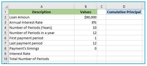
Let’s figure out the total principal paid over the course of the first year of a $90,000 loan using Excel’s CUMPRINC function. And at an interest rate of 8% each year, this loan must be fully repaid in 10 years. It is necessary to determine the loan’s monthly payment.
The starting period and end period values are as follows since the cumulative principal amount is to be established on the first year:
start_period = 1
end_period = 12
How to use Excel’s CUMPRINC function is shown below:
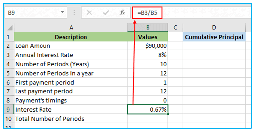
Step 1: Enter the following formula in cell B9 to calculate the monthly interest rate.
=B3/B5
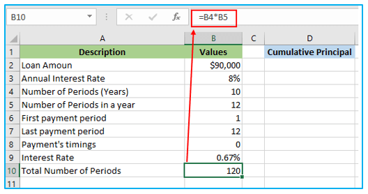
Step 2: Enter the following formula in cell B10 to calculate the total number of Periods.
=B4*B5
Step 3: Enter the following formula in cell D2 to calculate the cumulative principal amount paid during the first year of the loan.
=CUMPRINC(B9,B10,B2,B6,B7,B8)
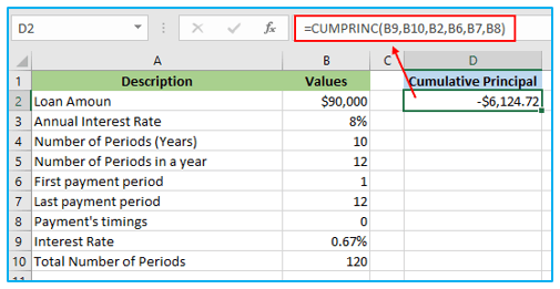
Since the principal paid is an outgoing cash flow, the CUMPRINC function’s output is a negative value.
Calculate the cumulative principal amount paid during the 4th year using the CUMPRINC formula in Excel:
Cumulative Principal Paid in 4th Year = CUMPRINC(Monthly Interest Rate, Number of Monthly Payments, Loan Amount, Start Period, End Period)
Since each year consists of 12 months, the 4th year would cover the period from the 37th month (start of the 4th year) to the 48th month (end of the 4th year).
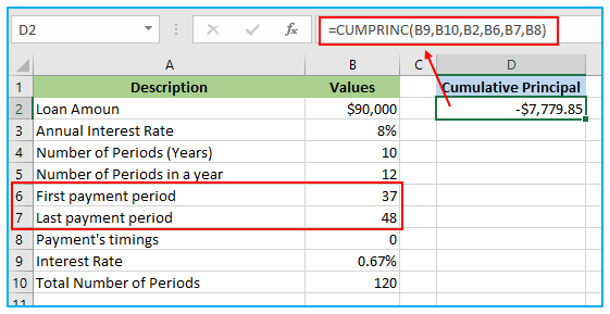
The total principal amount paid throughout the course of the fourth year is
CUMPRINC= -$7,779.85
The CUMPRINC function’s output is negative since the principal payment represents outgoing cash flow.
Please note that the cumulative principal amount will be calculated based on the actual payments made during the 4th year, so it may not be equal to the original loan amount divided by the number of years. It will depend on the actual payment schedule and the interest accrued during the previous years.
3. CUMPRINC Tips & Tricks:
Here are some helpful tips and tricks to maximize the utility of the CUMPRINC function in Excel:
- Payment Frequency Adjustment: When dealing with monthly payments, adjust the annual interest rate by dividing it by 12 and multiply the number of years by 12 to match the payment frequency. For quarterly payments, divide the interest rate by 4 and multiply the number of years by 4.
- Cumulative Interest Calculation: If you need to calculate the cumulative interest paid over a specific period, utilize the CUMIPMT function in Excel. This function complements CUMPRINC and helps you analyze the interest portion of loan payments.
- Remaining Balance Calculation: To determine the remaining balance of a loan after a particular period, leverage the FV function in Excel. This enables you to understand how much principal is yet to be paid off at any given point during the loan term.
- Principal Payment Calculation: For calculating the principal payment for a specific period, the PPMT function in Excel comes in handy. It isolates the principal component of loan payments, offering valuable insights into your repayment progress.
By employing these tips and using the appropriate financial functions in Excel, you can efficiently manage loan calculations, gain deeper financial insights, and make informed decisions regarding your debts and investments.
4. Common mistakes when using CUMPRINC:
Here are some common mistakes to be mindful of when using the Excel CUMPRINC function:
Payment Frequency Misalignment: Failing to adjust the interest rate and number of periods to match the payment frequency can result in inaccurate calculations. Always remember to divide the annual interest rate by the appropriate number (e.g., 12 for monthly payments) and multiply the total number of years accordingly.
Incorrect Type Argument: Using the wrong value for the type argument can lead to erroneous results. Keep in mind that 0 represents payments due at the end of the period (most common), while 1 signifies payments due at the beginning of the period.
Negative Present Value (pv): Providing negative values for the present value (pv) argument is a common mistake. The pv argument should always be a positive value, representing the initial loan amount or investment.
To ensure accurate calculations and reliable financial insights when using the CUMPRINC function in Excel, be cautious of these potential pitfalls and double-check your input values before executing the formula.
5. Why isn’t CUMPRINC Function working?
Consider the following troubleshooting methods if you run across problems with the CUMPRINC function:
Verify Required Arguments: Double-check that all necessary arguments for the CUMPRINC function are provided and in the correct format. Missing or incorrectly formatted inputs can lead to calculation errors.
Adjust Interest Rate and Periods: Ensure that you adjust the interest rate and total number of periods to match the payment frequency. Divide the annual interest rate appropriately (e.g., by 12 for monthly payments) and multiply the total number of years accordingly.
Check Type Argument: Verify that the type argument has the correct value (0 or 1) based on when the payments are due. Using the wrong type can result in inaccurate principal calculations.
Positive Present Value (pv): Make sure to use a positive value for the present value (pv) argument, representing the initial loan amount or investment. Providing a negative value can lead to unexpected results.
By following these troubleshooting steps, you can identify and rectify any issues that may arise when using the Excel CUMPRINC formula. This will help you obtain reliable and precise results for your loan principal payment calculations.
6. CUMPRINC: Related Formulae:
Related Formulas for Loan and Investment Calculations:
CUMIPMT: Use CUMIPMT to determine the total amount of interest paid over a given time period on a loan or investment.
FV: Utilize the FV formula to determine the future value of an investment based on periodic, constant payments, and a fixed interest rate.
PPMT: Employ PPMT to calculate the principal payment for a particular period of a loan or investment.
IPMT: Use IPMT to calculate the interest payment for a specific period of a loan or investment.
PMT: Leverage the PMT formula to calculate the periodic payment for a loan or investment, considering constant payments and a fixed interest rate.
These related formulas complement the CUMPRINC function and offer a comprehensive set of tools for various financial calculations, enabling you to make informed decisions and effectively manage loans and investments.
Application of CUMPRINC Function in Excel
- Loan Amortization: CUMPRINC Function in Excel calculates cumulative principal payments on a loan over its term, aiding in loan amortization analysis.
- Budgeting: Users can utilize this function to forecast and budget for principal repayments, helping in financial planning and management.
- Loan Repayment Analysis: It assists in analyzing loan repayment schedules by tracking the cumulative principal paid over time.
- Financial Modeling: CUMPRINC Function is valuable in financial modeling to project the impact of principal payments on cash flow.
- Debt Management: Users can monitor and manage debt effectively by understanding the cumulative principal payments required over time.
- Decision-making: This function aids in making informed financial decisions by providing insights into the principal portion of loan repayments.
You may be interested:
