CHOOSE function in Excel is a powerful tool for selecting values from a list based on an index number. It enhances data analysis, simplifies decision-making formulas, and improves workflow efficiency. By using the CHOOSE function effectively, you can streamline complex calculations and optimize your spreadsheets for better data management.
- What are the Excel CHOOSE function – syntax and basic uses
- How to use CHOOSE as an alternative to nested IFs in Excel? Example-1
- How to use CHOOSE as an alternative to nested IFs in Excel? Example-2
- How to use CHOOSE formula to generate random data in Excel?
- How to use CHOOSE formula to do a left VLOOKUP in Excel?
- How to use CHOOSE formula to return next working day in Excel?
- Notes about CHOOSE function.
1. What are the Excel CHOOSE function – syntax and basic uses.
By selecting “choose” in Excel, you can retrieve the position of the list’s value. Functions available in Excel 365, Excel 2019, Excel 2016, Excel 2013, Excel 2010 and Excel 2007
Syntax of the CHOOSE function is: CHOOSE(index_num, value1, [value2], …)
Index_num (required)- It returns the position of. This is either a reference, cell, or other formula within the range of 1 to 254.
Value1, value2, … – A list of 254 values to choose from. 1 must be used, while other values are not. The determination could be based on the number, text value, reference, formula, or name itself.
2. How to use CHOOSE as an alternative to nested IFs in Excel?
In Excel, it is common to return different values depending on the condition being entered. Declarations can be accomplished by utilizing classic, nested ones. However, some events are quick and easy to navigate.
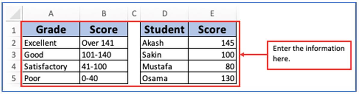
Step 1: Let’s say you have a list of Result grade and score grade and D column that features student name and E column student scores, here you want to marked the scores, as per the criteria provided:
The above information is writing here.
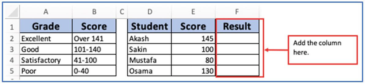
Step 2: Add the column from F1:F5 to get the result there.
The column has been added you can see it below.
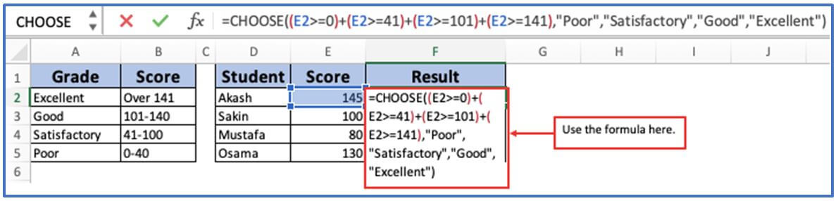
Step 3: Now, use the CHOOSE formula to get the result. Formula:
=CHOOSE((E2>=0)+(E2>=41)+(E2>=101)+(E2>=141),””Poor”,”Satisfactory”,”Good”,”Excellent”)
Applying the formula here.
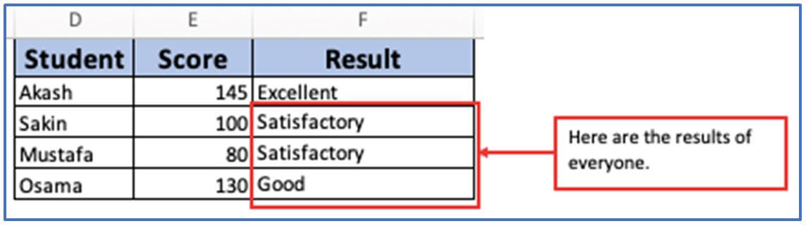
Step 4: After entering the formula press enter and the result will come out.
Akash’s result is outlined, the results is Excellent.

Step 5: It’s time to copy this formula into the remaining cells of the column. Just double-click or hold the fill handle and drag it down (located at the bottom right of cell here F2).
Here are all the results.
3. How to use CHOOSE as an alternative to nested IFs in Excel? Example-2
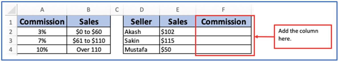
Step 1: Here given, the sales in amount and the commission in percentage also the Seller name and how much amount they sales. The percentage of commission will receive for selling a certain amount of money.
The data is placing here below.

Step 2: Now, you want to get the Commission for this add the column in F1:F4.
The columns have been added here.
Step 3: Now, you need to use the formula. The formula will be: =CHOOSE((E2>=0)+(E2>=61)+(E2>=110),E2*3%,E2*7%,E2*10%)
Using the formula here.

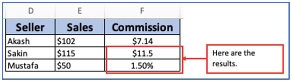
Step 4: Now, press Enter and you will get the Commission here.
The result is shown in the image.

Step 5: Now, use the same formula from Step-3 for the rest columns changing with the column range.
Here are all the Commission amounts.
4. How to use CHOOSE Formula to generate random data in Excel?
The RANDBETWEEN specified bottom and top numbers is created using Microsoft Excel’s “RANDBETWEEN Function” including the selection of index_num in your expression will result in almost all random data being generated.
Step 1: Select column A1 and give the column a name as Output.
Selecting the column here.

Step 2: Now add the column in A2:A6 to generate random data.
Adding the column here below.

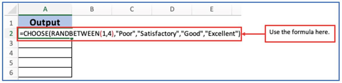
Step 3: Now use the formula. The formula: =CHOOSE(RANDBETWEEN(1,4),”Poor”,”Satisfactory”,”Good”,”Excellent”)
By generating random numbers from 1 to 4 RANDBETWEEN Function chooses the value from a list of four available values.
Applying the formula here.
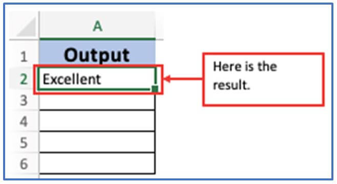
Step 4: Press enter and the result will come out.
Here is the result.
Step 5: now, drag-down the cursor from A2:A6.
The RANDBETWEEN function calculates all changes that you make to the spreadsheet, situated between the two. Hence, the list of your random numbers will also undergo modifications. Preventing this from happening by substituting the formulas with their values using a special paste feature.
Here are the outputs.

5. How to use CHOOSE formula to do a left VLOOKUP in Excel?
Excel allows you to search for objects in the left column, and if you perform an upright search, your selection will be displayed in that column. When the search column’s value needs to be left, you can opt for the Index /Match or Trick VLOOKUP combination by selecting.
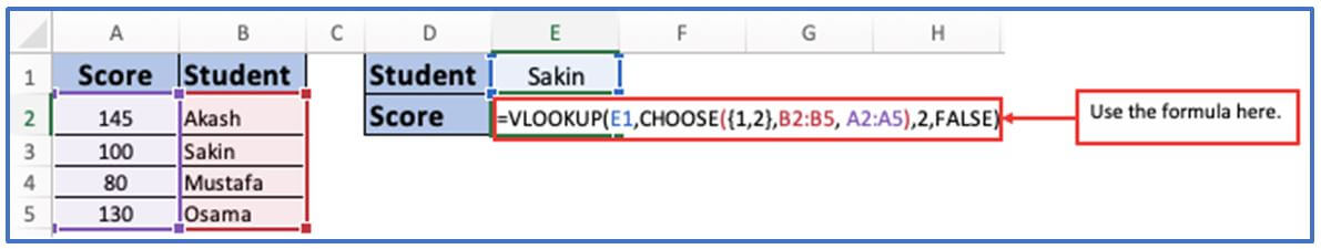
Step 1: Given that column A contains Scores and column B contains the Names of all the students. First make a list by writing the names and scores then enter that data into the table as shown below.
Here Placing the information into Excel.

Step 2: You want to get a specific Students score in one place. For this add the column in D1,D2 and E1,E2.
The column has been added here.

Step 3: You need to write down the formula now. Use this formula: =VLOOKUP(E1,CHOOSE({1,2},B2:B5, A2:A5),2,FALSE)
The formula has been applied here.
Step 4: Press enter and the result will come out. Here is the result after using the formula.
You can see Sakin score is outlined below. Here is the result.

6. How to use CHOOSE formula to return next working day in Excel?
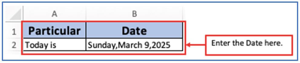
Step 1: First, input todays date into the excel as displayed.
Today’s date has been entered here.
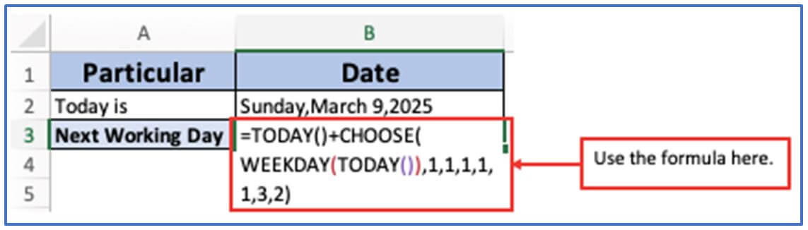
Step 2: Now, add the columns in A3 and B3 to get the next working day.
Adding the column here.

Step 3: The number that are returned for each day of the week is from 1 (Sunday) to 7 (SAT) The index_num argument of our chosen formula is denoted by this number.Value1 – Value7 (11,1,1,3,2) Determine the number of days added on the current day If today is Sunday – Thursday (index_num 1 – 5), you will add 1 to return the next day If today is Friday (index_num 6), you will add 3 to return next Monday If today is Saturday (index_num 7), you will add 2 to return on Monday.
To get next working day use this formula: =TODAY()+CHOOSE(WEEKDAY(TODAY()),1,1,1,1,1,3,2)
Using the formula below.
Step 4: When the formula is set, press enter and the result will come out.
Here is the result of next working day outlined below.

7. Notes about CHOOSE function.
- VALUE! Error –If you specify a number that is less than or equal to 1, the specified index_num will be used instead. The specified index argument is not a numerical value.
#NAME?Error – Happens when the value argument is not enclosed in quotation marks and is a text value that cannot be used as arbitrary reference for cell.
Application of CHOOSE function in excel
- Selecting Values from a List – Picks a value from a predefined list based on a given index number.
- Creating Dynamic Drop-Downs – Helps in generating dynamic lists without needing complex IF statements.
- Choosing Data for Calculations – Selects specific datasets to perform calculations, making formulas more efficient.
- Simulating Conditional Logic – Acts as an alternative to nested IFs by selecting different values based on conditions.
- Generating Randomized Outputs – Can be used with the RANDBETWEEN function to return random selections from a list.
- Custom Sorting of Data – Helps in rearranging data dynamically by picking values in a custom order.
For ready-to-use Dashboard Templates:
