How to use 3D formula in Excel?

3D formula in Excel is a powerful tool that allows users to reference and analyze data across multiple worksheets in a workbook. By using a 3D formula, you can perform calculations over several sheets with a simple reference to the range of sheets, making it easier to summarize data from different parts of a workbook. This method enhances the efficiency of complex calculations and helps keep your workbook organized. Whether you’re working with large datasets or multiple categories, the 3D formula can significantly improve your workflow and data analysis process.

What is an Excel 3-D reference?
How to Create a 3D reference in Excel? Example-1
How to Create a 3D reference in Excel? Example-2
How to create a chart with 3D Reference in excel?
How do Excel 3D references change when you insert, move or delete sheets in excel?
Things you should keep in mind while doing 3D reference

1. What is an Excel 3-D reference?

The ability to refer to the same cell or range of cells in Excel 3D allows you to do so across multiple worksheets. It’s not just about any number of cells, it also has a variety of worksheet names. It is essential to ensure that all referenced sheets possess the same model and data type.

The term “3D reference” in Excel is a formula that can be used across multiple worksheets, enabling you to refer to the same cell or range on different worksheet sheets in. It can be beneficial when you have similar information distributed among several worksheets and need to compute for each of them. Data from multiple worksheets, or cells, is consolidated into a single calculation using data contained within overlapping 3D references.

2. How to Create a 3D reference in Excel? Example-1

Step 1: Enter Black coffee, Milk, tea as item and add 3 Quarters as shown below.

The data has been placed here.

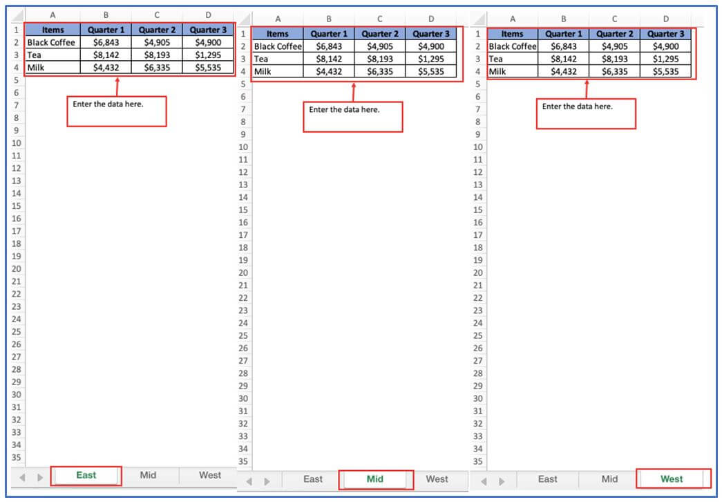
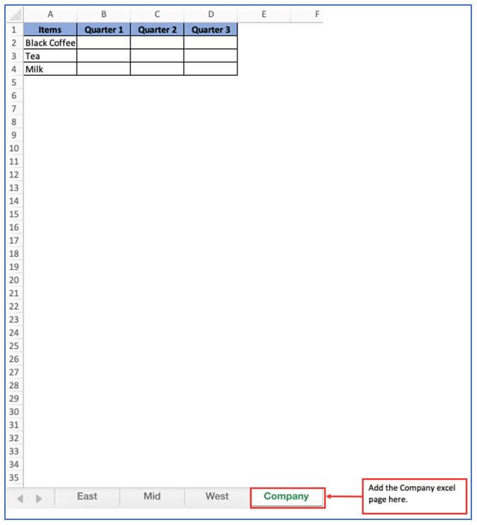
Step 2: Now add another page to Calculate of East excel page quarter 1(B2), Mid excel page quarter 1(B2) and West excel page quarter 1(B2) these 3 places quarter 1 should be done on company page together in Quarter 1.

The company page has been added.

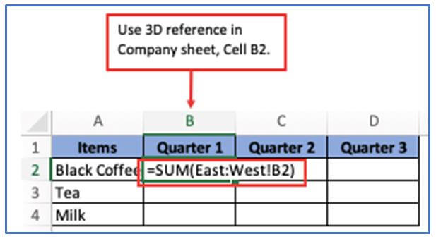
Step 3: Use the 3D reference North: South instead. To address the SUM function. 3D reference is: =SUM(East:West!B2)

Using the 3D reference here below.

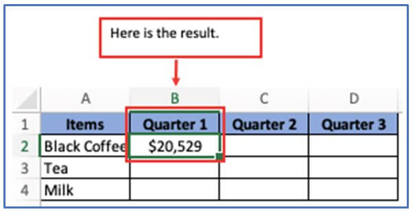
Step 4: The addition of the North and South panels to the formula in cell B2 will automatically include them. Here is the sum of Every sheet cell B2, Quarter 1. You can follow the same 3D reference from Step-3 changing with cell number for the rest of the items and Quarters.

Here is the result below.

3. How to Create a 3D reference in Excel? Example-2

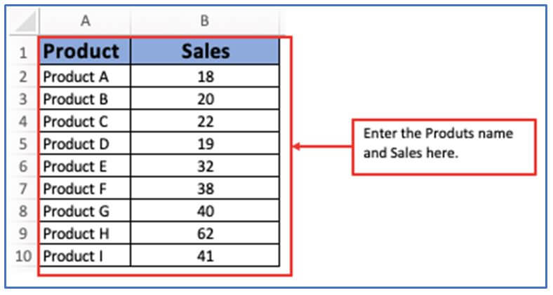
Step-1: First make 2 sheets in the excel sheet. Sheet 1 contains the price list of products, while sheet 2 is titled “Products sold” to display the number of items that have been sold.

Input all the above information into the excel as shown below.

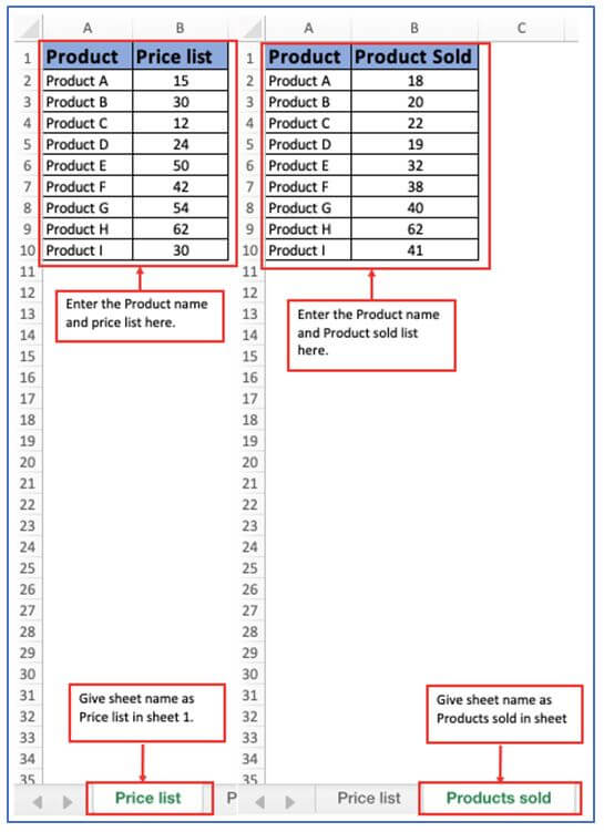
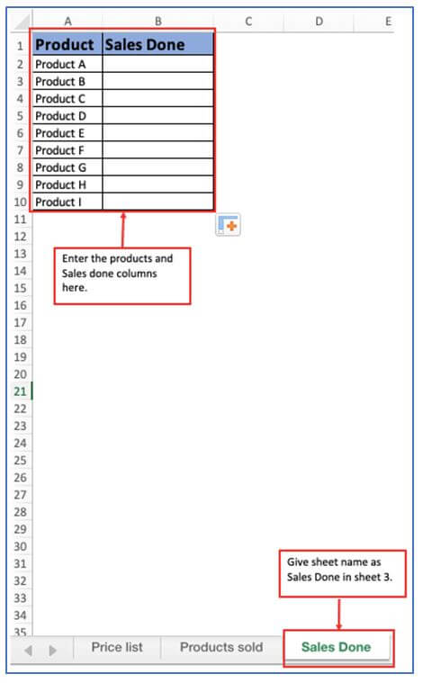
Step 2: Now add another sheet. In Sheet 3, here will calculate the sales of the product and rename it as “Sales Done.

Sheet 3 have been added.

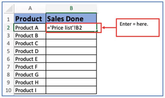
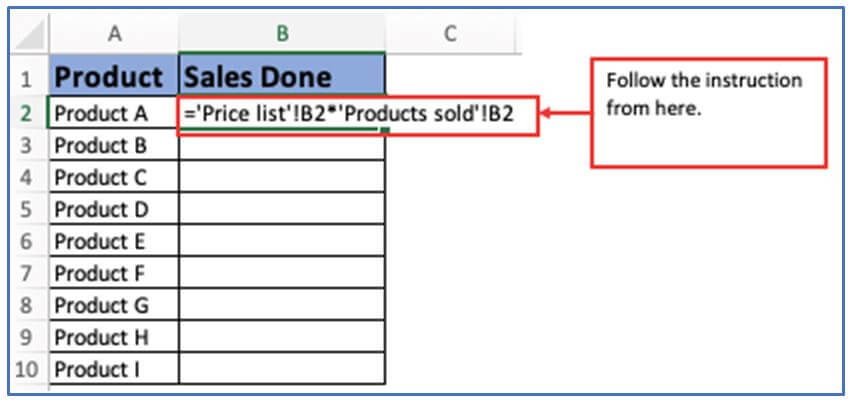
Step 3: Type the formula “=” in cell B2, sheet 3(Sales done), then suggest to sheet 1-a price list. Afterward, choose the price for the first product, product A.

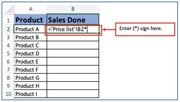
Step 4: You can see that the Excel toolbar refers to the first price list in cell B2 in sheet 3(Sales done). You can now use an asterisk (*) to indicate multiplication in Excel.

Using the asterisk (*) sign below.

Step 5: Now turn to sheet 2, one product sold. In cell B2, find the number of products sold.

Following the above instruction below.

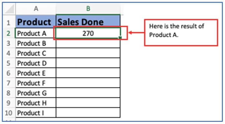
Step 6: Excel’s toolbar displays products sold in cell B2 as the second sheet. Tap the button to enter. Here has the revenue available for product A, as a result.

Here is the result of Product-A.

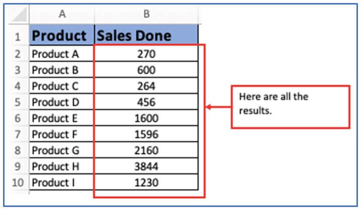
Step 7: Now drag the formula to cell B2 to B10. By using the corresponding price list and the number of products sold, Excel can automatically calculate the sales figures for other products.

Here are all the sales done results.

4. How to create a chart with 3D Reference in excel?

Step-1: Here, given a spreadsheet with sales data.

The information presented is as follows.

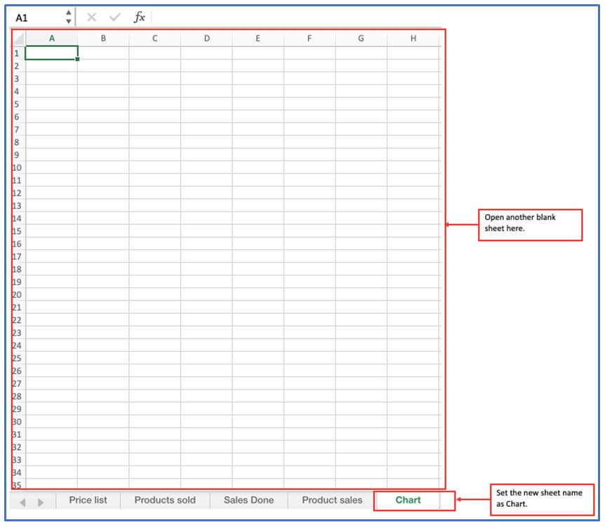
Step 2: Now add another sheet for making the chart and name as chart.

Another sheet has been added.

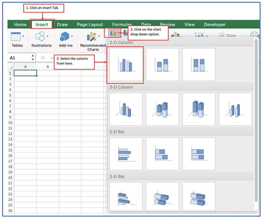
Step 3: Using the same data, here will generate a chart in another spreadsheet. Choose from a variety of chart choices in another worksheet. Go Insert>Chart drop down box. Here picked a 2D Column Chart.

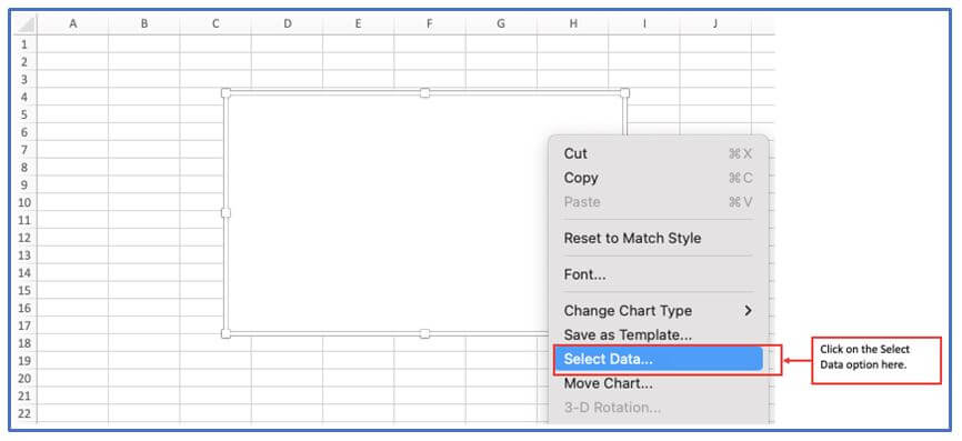
Step 4: After choosing 2D column chart a blank chart appears. After that, click on the appropriate button and then choose “Select Data” to proceed.

Step 5: An opening dialog box will be displayed. Now, pick the data for company sales from the other sheet and enter it in the chart data range.

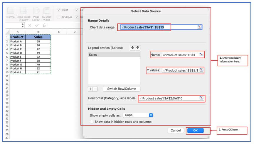
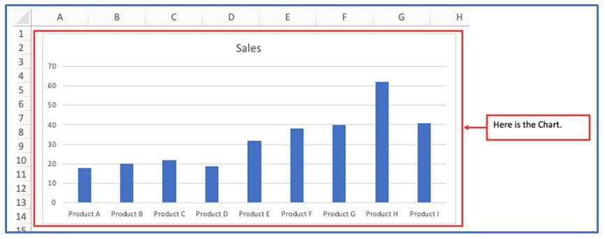
Step 6: Here generated the chosen chart in the other sheet by clicking on “OK”. By utilizing 3D reference, here have created the chart successfully.

Here is the chart below.

5. What are the List of functions supporting 3D references in Excel?

Here is the list of Excel Functions that permit applying 3D references.

SUM	It adds up numerical values.
AVERAGE	It calculates arithmetic mean of values, including numbers, text and logical.
COUNT	It Counts cells with numbers.
COUNTA	It Counts non-empty cells.
MAX	It Returns the largest value.
MAXA	It Returns the largest value, including text and logical.
MIN	It Finds the smallest value.
MINA	It Finds the smallest value, including text and logical.
PRODUCT	It Multiplies numbers.
TEXTJOIN	It combines values from multiple cells into one with a specified delimiter.
STDEV, STDEVA, STDEVP, STDEVPA	It Calculate a sample deviation of a specified set of values.
VAR,VARA, VARP, VARPA	It Returns a sample variance of a specified set of values.

6. Things you should keep in mind while doing 3D reference

while using 3D references in Excel, there are a few important points to keep in mind:

Consistent data structure:The referenced cell or range must exist in the same location in all worksheets. If the structure is different, the results may be incorrect or incomplete
Naming tables:Make sure the tables you reference have consistent and correct names. The range specified by Excel will only include sheets that match it, such as “January”
Order of sheets: The order in which the sheets are cited is contingent on their reference. Whether you move a sheet in the referenced range or not, will produce different results. Make sure the sheets are in the correct order
Hidden Sheets:Excel will automatically add values from hidden sheets to the 3D reference, so be cautious if you hide certain sheets.
Sheet addition or removal: The calculation will automatically include sheets from the referenced range if they are added, and those from removal will be removed from their reference.
Limitations on certain functions:Certain 3D references are compatible with only Excel functions like SUM (), AVERAGE () and MAX (Some functions, like VLOOKUP () or MATCH () are not able to provide 3D references.
Detailed explanations: Be careful with circular references, where a formula accidentally references itself in multiple worksheets errors and performance issues can result from this.

When you take into account these factors, you can use 3D references in Excel with precision and efficiency.

Application of 3D formula in Excel

Consolidating Data Across Multiple Sheets: The 3D formula allows you to reference the same cell or range across multiple worksheets, which is useful for consolidating data from different periods or categories in a single calculation.
Summing Data from Multiple Sheets: You can use a 3D formula to sum the same range of data across several sheets, making it easier to calculate totals for similar data across different sheets, like monthly sales data.
Comparing Data Across Worksheets: The 3D formula enables you to compare values from corresponding cells in multiple worksheets, helping you spot trends or anomalies.
Automating Financial Reports: You can use a 3D formula to automate the generation of reports by referencing cells across different sheets, which can save time in financial analysis and budgeting.
Performing Group Calculations: When working with multiple worksheets that represent different groups or categories, 3D formulas allow you to calculate statistics like averages or sums across those groups.
Data Analysis in Large Workbooks: For large workbooks with many sheets, the 3D formula makes it possible to perform complex calculations and data analysis without the need for manual input from each sheet individually.

For ready-to-use Dashboard Templates: