SUM by Color in Excel is a powerful technique for enhancing your data organization and analysis. By utilizing this function, you can quickly aggregate and assess data based on color-coded categories, enabling clearer insights and more strategic decision-making. Whether you’re managing budgets, tracking sales performance, or monitoring inventory levels, incorporating SUM by Color into your Excel toolkit can significantly streamline your processes and improve your understanding of complex datasets. Embrace this feature to bring efficiency and clarity to your spreadsheets, transforming color-coded data into actionable intelligence.
This Tutorial Covers:
- How to SUM by Color in Excel?
- How to SUM by Color by using SUMIF Function? / Excel SUMIF Function to Get Sum of Columns by Color.
- How to SUM by Color by using the SUBTOTAL Function?
- How to SUM by Color using Get Cell Function?
- How to SUM by Color Using Excel Table Design?
1. How to SUM by Color in Excel?
Excel has some fantastic functions, but none of them can sum cells by color. When working with Microsoft Excel, we use different fill colors to help us understand the data in the cells. Eventually, we’ll need to compute the sum-colored cells in excel. Unfortunately, there is no straightforward way to compute the sum of cell values in columns. Now, I’ll go over a few methods for completing the calculation.
2. How to SUM by Color by using SUMIF Function?
To sum by Color by using SUMIF Function, follow the process:
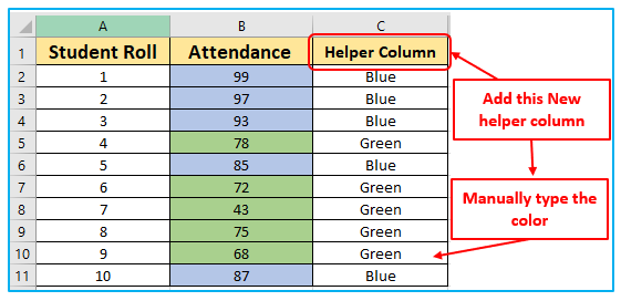
Step 1: To the main dataset, add a helper column and manually type the color of the cells.
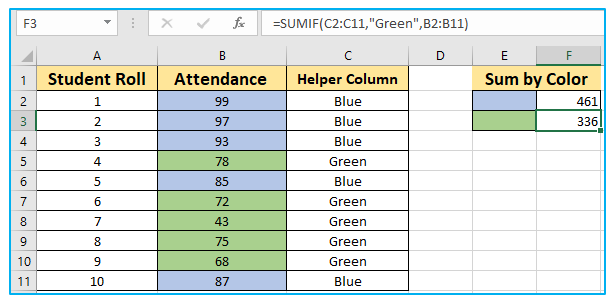
Step 2: Enter the following formula in cell F2:
The following formula can be used to sum by Color:
=SUMIF(C2:C11,”Blue”,B2:B11)

Step 3: Likewise, use the formula below to calculate the total number of Green-colored cells.
=SUMIF(C2:C11,”Green”,B2:B11)

Results are outlined below:
3. How to SUM by Color by using the SUBTOTAL Function?
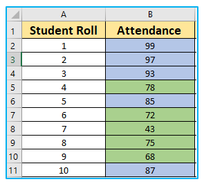
Below I have a dataset where I have the student roll numbers and their attendance.
Step-1: Enter the following formula in the cell where you want the sum result. I will enter the formula in cell B3.
=SUBTOTAL(9,B2:B11)
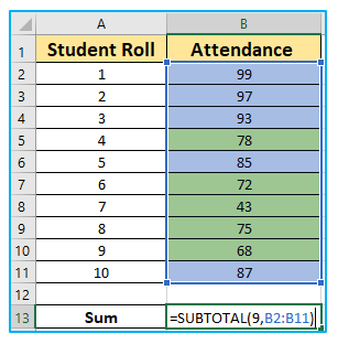
The number 9 in the function num argument denotes sum functionality, and the reference argument specifies the range of cells to be computed.
Result of the Subtotal Function:
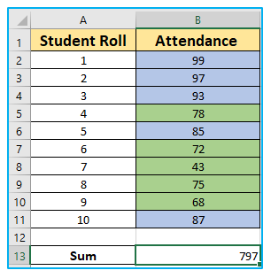
Step 2: Now, Select any cell in the dataset.
Step 3: By going to the “Data” tab and selecting a filter, you can apply the filter to the data table.
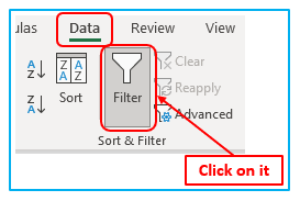
Step 4: After applying the Filter, click on the drop-down menu of the Attendance column.
Step-5: Then, click Filter by Color and select any color from the Filter by Cell Color menu. Blue is the color I’ve chosen.
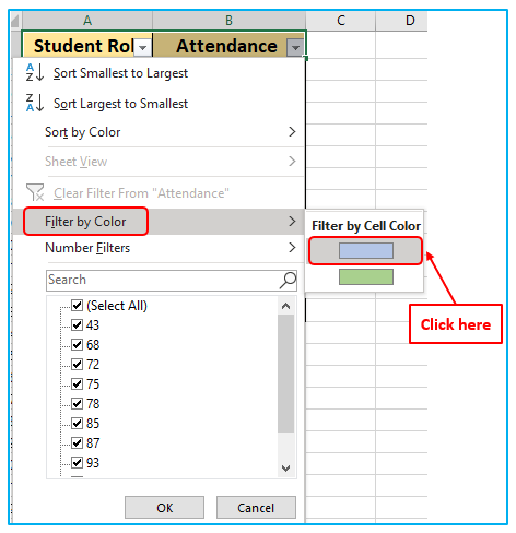
Results are outlined below:
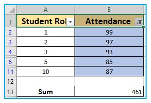
Similarly, if you filter the data set by a different color, the SUBTOTAL function will adjust and return the sum of all cells with the desired color.
4. How to SUM by Color using Get.Cell Function?
To find the color indexes of the cell colors used in columns, we will use the GET.CELL function. And after that, we’ll use the SUMIF function to compute the summation based on a specific color.
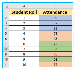
Below I’ve attached a dataset with colored cells that I’d like to sum.
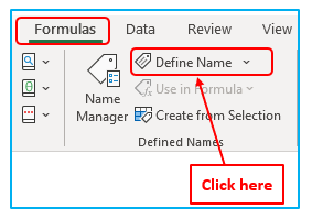
Step-1: In the Ribbon, click the Formulas tab, then in the Defined Names group, click the ‘Define Name.’
Step 2: The New Name dialog box will open. Fill in the Refers to box with a suitable name for your range and the formula. Then click OK to exit the Name Manager dialog.
The following formula can be used:
=GET.CELL(38,$B2)
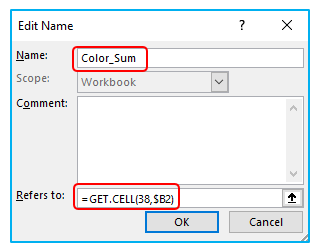
As shown in the screenshot above, the function’s name is “Color_Sum,” and the formula (=GET.CELL(38,$B2)) is to be entered in the ‘Refers to’ field. The numeric 38 refers to the cell code information within the formula, and the second argument is the cell number B2, which refers to the reference cell.
Step 3: To list the color indexes, add an extra column beside the Attendance cell. In Cell C2, enter the range’s name.
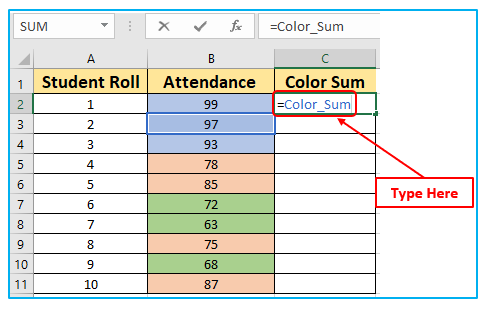
Step 4: Use the same formula for all of the cells in column C. Fill in the blanks with the fill handle or simply copy and paste cell C2.
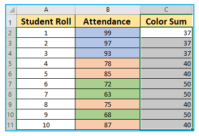
We can use the SUM of cells based on their color now that we have a unique number for each color.
Step-5: In Cell F2, enter the SUMIF formula and press Enter.
The following formula can be used:
=SUMIF(C2:C11,E2,B2:B11)
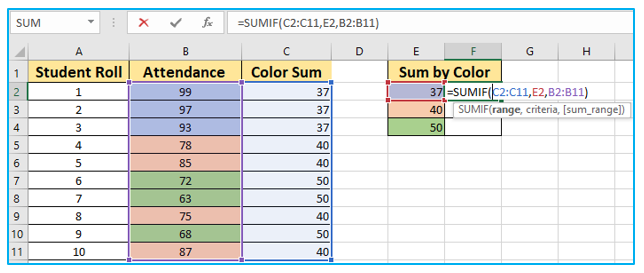
Step 6: For all of the color code numbers whose values are to be added together, the SUMIF formula is dragged down.
5. How to SUM by Color Using Excel Table Design?
Step-1: Convert the dataset into a table by pressing Ctrl +T.
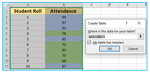
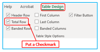
Step 2: The Table Design tab will appear after you select the table.
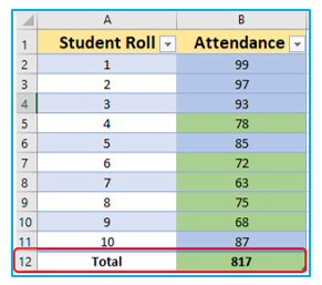
Step 3: Now, go to the Table Design tab and select the Total Row checkbox.
Step-4: It will give us the following total of all Attendance:
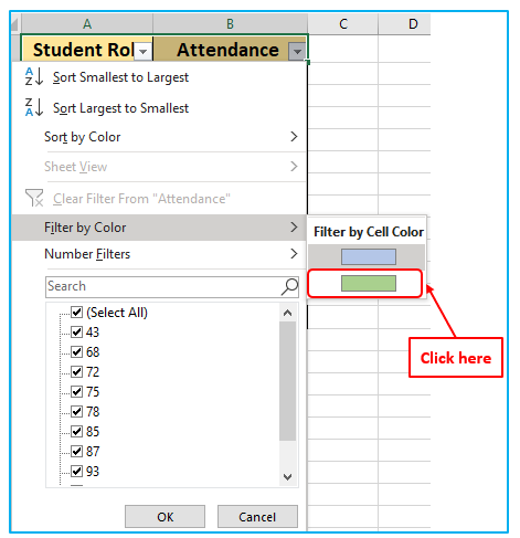
Step-5: Then, click Filter by Color and select any color from the Filter by Cell Color menu. Green is the color I’ve chosen.
Results are outlined below:
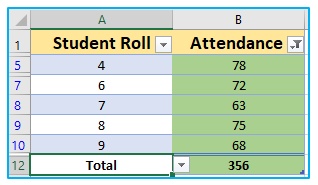
Similarly, if you filter the data set by a different color, the function will adjust and return the sum of all cells with the desired color.
Application of SUM by Color in Excel
- Project Budgeting: Sum expenses or incomes categorized by different colors, representing various categories (e.g., travel, supplies, labor) to track and manage project budgets efficiently.
- Sales Analysis: Aggregate sales data colored based on product types or regions to analyze performance metrics and identify best-selling products or most profitable markets.
- Performance Tracking: Sum values color-coded to represent different performance levels (e.g., green for above target, red for below target) to quickly assess team or individual performance.
- Inventory Management: Calculate the total of inventory items marked with different colors indicating status levels, such as in-stock (green), low stock (yellow), or out-of-stock (red), for effective inventory control.
- Event Planning: Tally up costs or resources for an event, categorizing each by color based on the type of expense or resource (e.g., venue, catering, entertainment) for better financial management.
- Educational Grading: Sum scores or points in grading sheets where colors represent different grading categories or levels (e.g., blue for tests, yellow for homework), simplifying grade calculation and analysis.
You may be interested:
