Sort Data by Color in Excel is a powerful feature that allows you to organize and analyze data visually. It goes beyond traditional sorting methods by using color to prioritize tasks, track statuses, and categorize data effortlessly. This function helps uncover patterns, trends, and insights that may have gone unnoticed. By utilizing this feature, you can enhance data organization and reporting, making your Excel worksheets more efficient and clear. Whether you’re managing projects, checking data quality, or improving data visualization, Sort Data by Color in Excel empowers you to extract meaning from color-coded information.
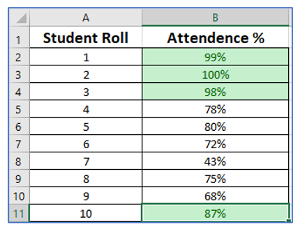
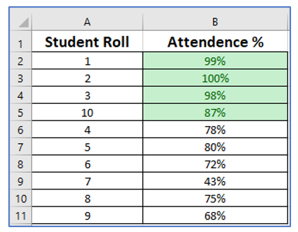
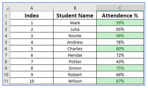
Given a dataset of student attendance. In the given data set the rows are colored with green whose attendances are greater than 85%. Try putting all the cells at the top whose attendance are greater than 85%.
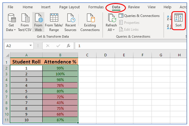
Steps for sorting data by single color:
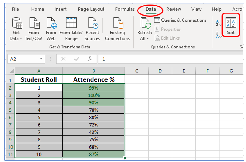
Step-1: Select the cells you want to apply the sort to. (Cells A2 to B11 in the example).
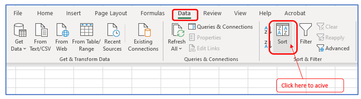
Step 2: Select the Data Tab and then select the Sort option. Choose Sort from the menu. This will bring up the Sort dialog box.
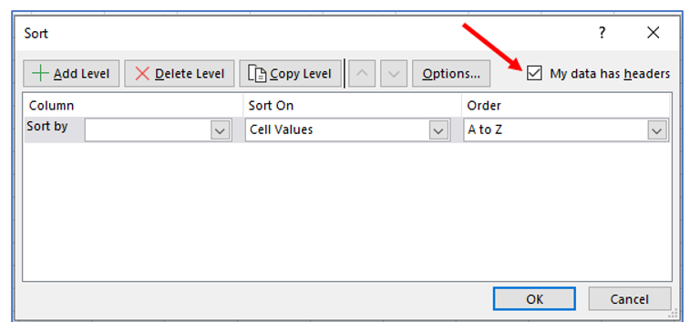
Step 3: Make sure “My Data has headers” is chosen in the Sort dialog box. You can leave this option unchecked if your data doesn’t include headers.
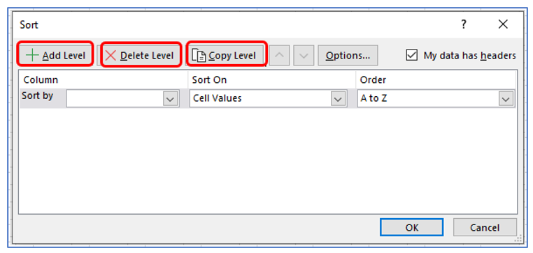
Step 4: There are multiple choices in the pop-up.
Add Level: Depending on the priority, we can add various levels using this option.
Delete Level: It aids in erasing the extra levels.
Copy Level: It enables us to duplicate various levels in order to reorganize the priority.
Step 5: Select the basis on which you wish to sort the data under Sort by column.
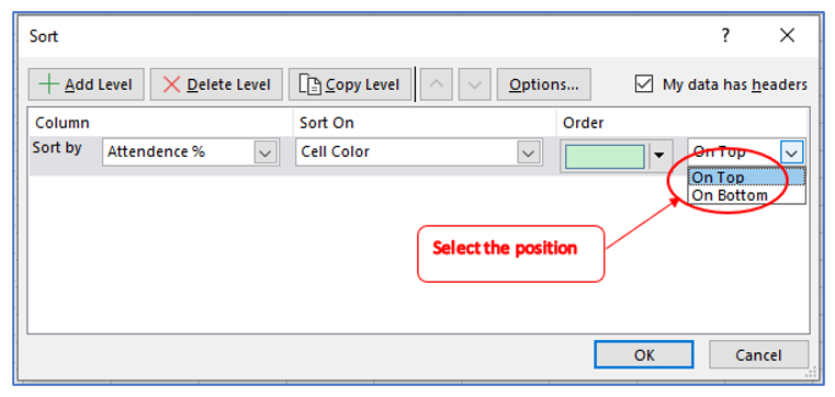
Step 6: Select “Cell Color” under “Sort On” to arrange your cells according to the color of their backgrounds.
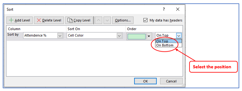
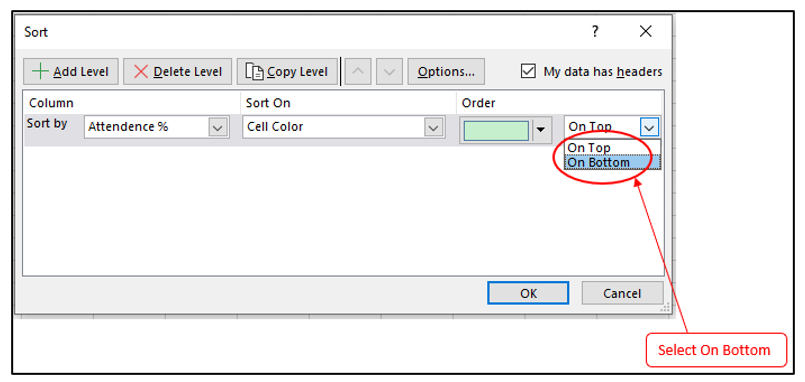
Step 7: Select the color you wish to retain at the top or bottom of the list by clicking the “Order” drop-down menu.
Step 8: Choose where you want to put the cells with the chosen color by clicking the drop-down menu next to this one. You have two choices: “On Top” and “On Bottom.”
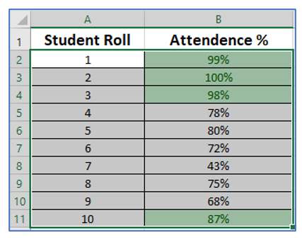
Step-9: Click OK. Result outlined below:
How to Sort by Multiple Color in Excel?
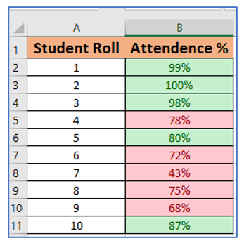
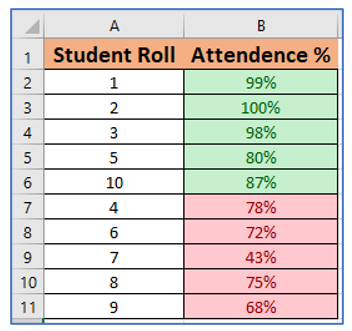
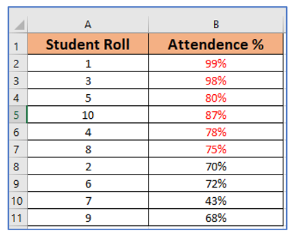
Given a dataset of Students attendances. In the given data set the rows are colored with green whose attendances are greater than 80% and red whose attendance are below 80%. Try putting all the cells at the top whose attendances are greater than 80%.
Steps for sorting data by Multiple color:
Step-1: Select the cells you want to apply the sort to. (Cells A2 to B11 in the example).
Step 2: Select the Data Tab and then select the Sort option. Choose Sort from the menu. This will bring up the Sort dialog box.
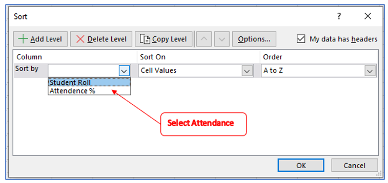
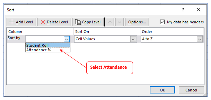
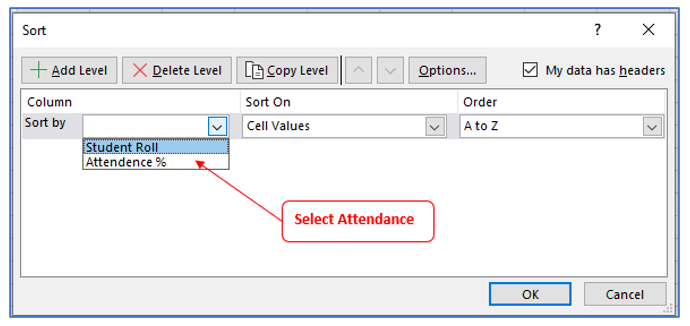
Step-3: Select “Attendance” from the “Sort By” drop-down menu. This is the column that we intend to use to sort the data.
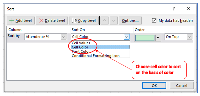
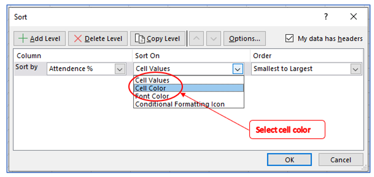
Step-4: Go to the ‘Sort On’ drop-down menu and select Cell Color.
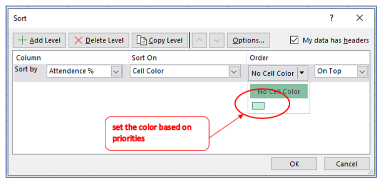
Step-5: Pick the first color you want to use to sort the data from the ‘Order’ drop-down. It will display each and every color found in the dataset. Choose green.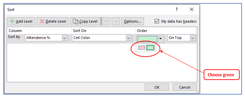
Step-6: Choose your first fill color and retain On Top for the Order value.
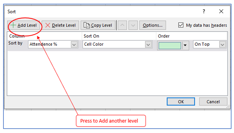
Step-7: In the panel’s upper left corner, click the Add Level button. This will result in the addition of another sort order rule.
Step 8: Select the basis on which you wish to sort the data under Sort by column.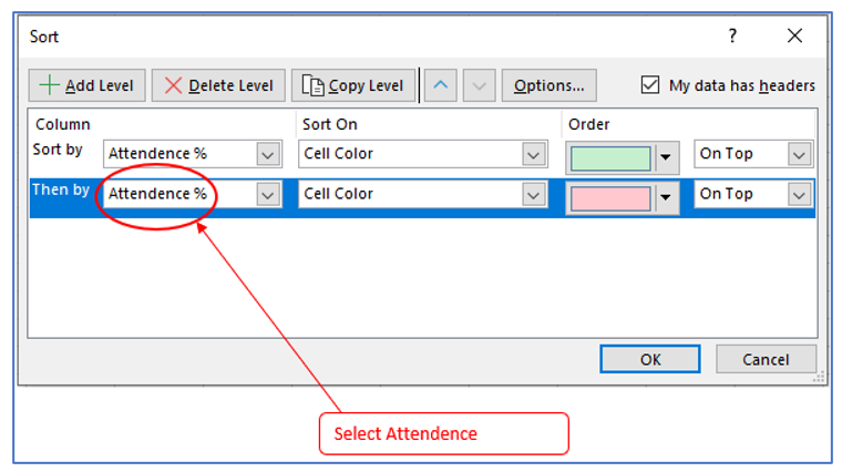
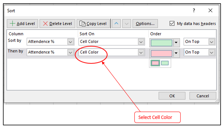
Step-9: Go to the ‘Sort On’ drop-down menu and select Cell Color.
Step-10: Select the second color you wish to use to sort the data in the ‘Order’ drop-down. It will display each and every color found in the dataset. Choose Red.
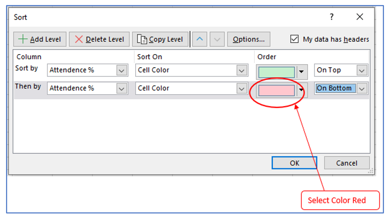
Step-11: Choose On-Bottom from the second drop-down menu under Order.
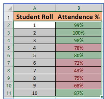
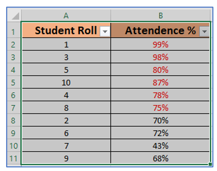
Step-12: Click OK. Result outlined below:
How to sort data by font color?
Steps for sorting by font color:
Step-1: Select the cells you want to apply the sort to. (Cells A1 to B11 in the example).
Step 2: Select the Data Tab and then select the Sort option. Choose Sort from the menu. This will bring up the Sort dialog box.
Step-3: Select “Attendance” from the “Sort By” drop-down menu.
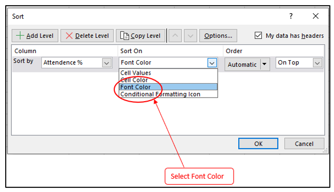
Step-4: Go to the ‘Sort On’ drop-down menu and select Font Color.
Step-5: Pick the red color to sort the data from the ‘Order’ drop-down.
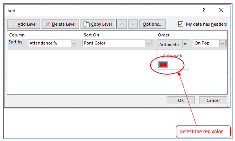
Step-6: Choose ‘On Top’ for the Order value.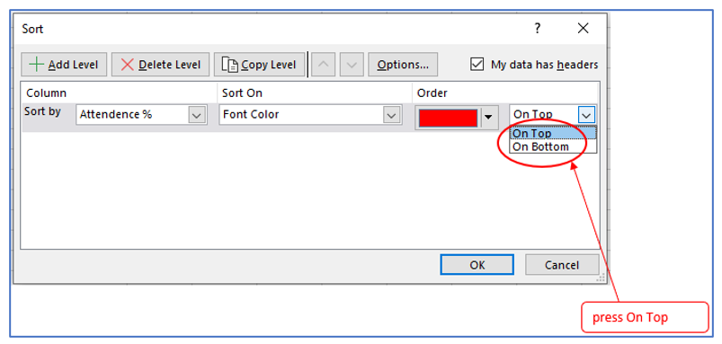
Step-7: Click OK. Result outlined below:
How to bring back original order of the data?
- You can easily restore the data to its initial state by using the Undo button (or the shortcut Ctrl + Z). However, you can only accomplish this if you do it immediately after applying filters. After much editing and closing and reopening of workbooks, this would not be a trustworthy way to employ.
- The most dependable technique is to temporarily add a new column with sequential numbering and then, to return to the initial condition, filter using the temporary ordinated column.
Steps for bringing back the original order of the data:
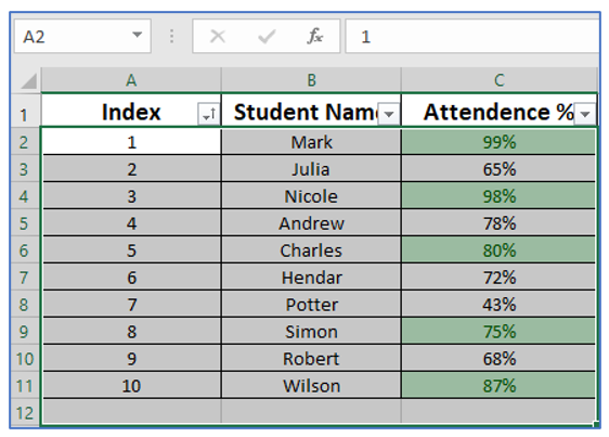
Step-1: Prepare a data table with sequential numbering outlined below:
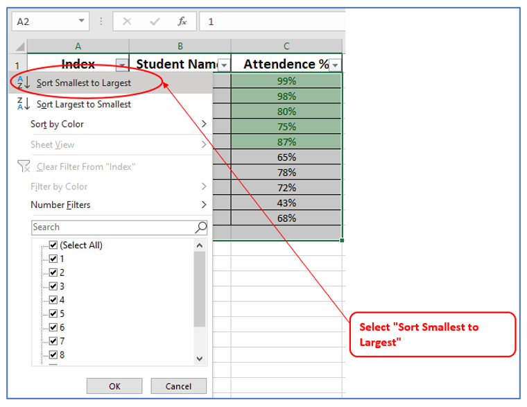
Step-2: After different Sorting, if you want to revert back, Select the Data Tab and then select the Filter option.
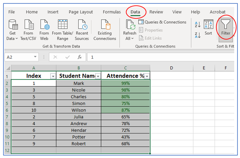
Step-3: Select the dropdown arrow appeared in Index cell.
Filter result will be appeared, outlined below:
Application of Sort data by Color in Excel
- Priority Tasks:
- Sort tasks or action items by color-coding them based on priority, allowing you to tackle high-priority items first.
- Status Tracking:
- Sort data by color to track the status of projects or tasks, easily identifying completed, ongoing, or overdue items.
- Categorization:
- Group and categorize data by color, such as organizing products into categories or grouping expenses by type.
- Data Quality Analysis:
- Sort data by color to identify and analyze data quality issues, such as missing or inconsistent data marked with specific colors.
- Conditional Formatting Insights:
- Sort by color to gain insights from conditional formatting rules, helping you spot trends or outliers in your data.
- Data Visualization:
- Sort and arrange data by color for effective data visualization, creating color-coded heatmaps or data representations for reports and dashboards.
Sorting data by color in Excel enhances data organization and analysis, enabling you to make informed decisions and gain insights from color-coded information.
For ready-to-use Dashboard Templates:
