How to sort by Multiple Columns in Excel?

Sort by Multiple Columns in Excel is a powerful feature that enables users to organize data systematically based on multiple criteria simultaneously. By leveraging this functionality, users can arrange data hierarchically, ensuring that primary sorting criteria take precedence while secondary criteria are applied as tiebreakers. Whether sorting data for analysis, reporting, or presentation purposes, the ability to sort by multiple columns in Excel enhances efficiency and improves data organization. This feature is particularly useful when dealing with complex datasets that require nuanced sorting to extract meaningful insights. With sort by Multiple Columns in Excel, users can streamline their data management workflows, increase productivity, and make informed decisions with confidence. Embrace the versatility and effectiveness of this feature to unlock the full potential of your Excel spreadsheets and enhance your data analysis capabilities.

This Tutorial Covers:

1. How to sort by one column
2. How to sort by multiple column
   • Using Sort dialog box
   • Using SORTBY Function
     • Syntax
     • Arguments
     • How to use SORTBY function

1. How to sort by one column?

Sorting data by one column in Excel is a straightforward process. Assume you own a dataset similar to the one below.

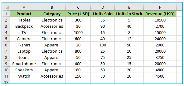
You can sort your Excel data in one column in ascending or descending order.

The steps to sort by one column in Excel are described below:

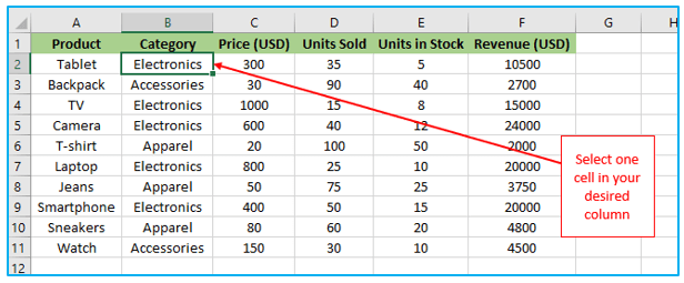
Step 1: To sort a column, click any cell in the desired column.

Step 2: Click “AZ” in the “Sort & Filter” group under “Sort & Filter” on the “Data” tab to sort in ascending order.

Result:

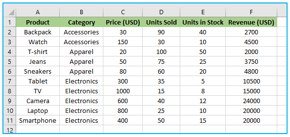
Note: Click ZA to sort in descending order.

2. How to sort by multiple column?

When dealing with complex datasets in Excel, you often encounter scenarios where sorting data based on just one column is not sufficient to fully analyze and make sense of the information. In such cases, sorting data by multiple columns becomes essential. By sorting data on multiple criteria simultaneously, you can effectively organize your data and gain deeper insights from it.

We will explore how to use the Sort dialog box in Excel to sort data by multiple columns using two methods, which are described in the next section.

• Using Sort dialog box:

You can add more levels to your data sort when utilizing the sort dialog box.

The steps to perform multi-level sorting using the dialog box are described below:

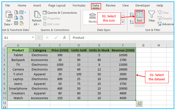
Step 1: Choose the whole collection of data you wish to sort.

On the Excel ribbon at the top of the window, select the “Data” tab. Simply select the “Sort” icon from the “Sort & Filter” group.

Step 2: Make the following selections in the Sort Dialogue box:

• Sort by (Column): Category (this is the first level of sorting)
• Sort On: Cell Values
• Order: A to Z

Make sure the “My data has headers” option is selected if your data contains headers.

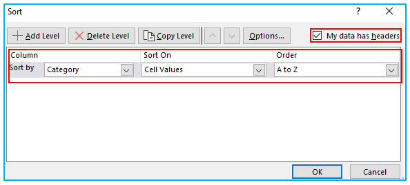
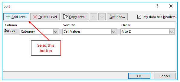
Step 3: The “Add Level” button must be clicked to add a new level of sorting choices.

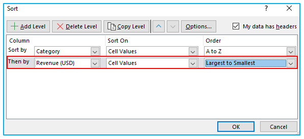
Step 4: Make the following decisions for the second level of sorting:

• Then by (Column): Takings (USD)
• Sort On: Cell Values
• Order: Largest to Smallest

Click OK

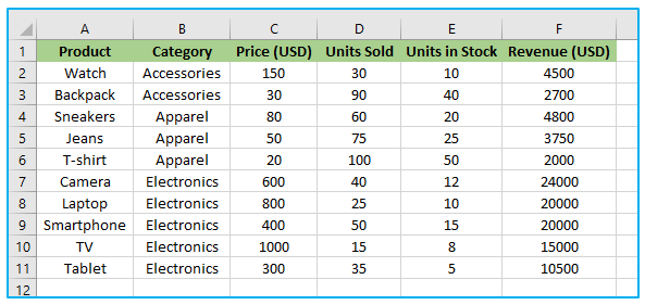
The results of the aforementioned steps are displayed below. The data is sorted first by category, then by the Revenue (USD) column. Be aware that the category column does not change when the Revenue (USD) column is sorted since the category column is sorted first.

• Using SORTBY Function:

The SORTBY function uses the values in the associated range or array to order the contents of a range or array.

Using the Excel SORTBY formula, you can sort multiple columns simultaneously and create sophisticated sorting rules to organize your data effectively.

• Syntax:

Following is the syntax for Excel’s SORTBY function:

=SORTBY(array, by_array1, [sort_order1], [by_array2, sort_order2], …)

• Arguments:

Following is the arguments for Excel’s SORTBY function:

array: This is the range of cells or array of values that you want to sort. It includes the data you want to rearrange based on the sorting criteria.

by_array1: This parameter represents the range or array you want to sort the data by. It defines the primary sorting criteria.

[sort_order1]: This is an optional parameter that specifies the sort order for the first “by_array.” Use 1 for ascending order and -1 for descending order.

[by_array2, sort_order2]: These are optional parameters that allow you to include additional sorting criteria. You can use multiple “by_array” and “sort_order” pairs to create a hierarchical sorting order.

Note: Please ensure that you have the latest version of Excel or a Microsoft 365 subscription to access the SORTBY function, as it may not be available in older versions of Excel.

• How to use SORTBY function?

Assume you own the same dataset as used in the previous example, similar to the one below.

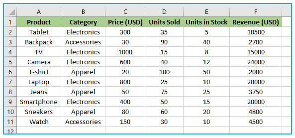
The steps to use SORTBY function in Excel are described below:

Step 1: First of all, create a header in the same sheet, another new sheet, or another new workbook, as you wish. In this example, we created the header on the same sheet.

Step 2: Enter the following formula in cell H2.

=SORTBY(A2:F11,B2:B11, 1,F2:F11, -1)

Let’s analyze the formula and explain each of the parts in turn:

A2:F11: This is the range of cells that contain the data to be sorted. It includes all the columns from A to F and all the rows from 2 to 11. The data in this range will be rearranged based on the specified sorting criteria.

B2:B11: This represents the first “by_array” parameter, which is the range to sort by. In this formula, we are using the values in column B (cells B2 to B11) to determine the primary sorting order.

1: This is the “sort_order1” parameter and is optional. In this case, we’ve used 1 to indicate ascending order. This means that the data will be sorted based on the values in column B (range B2:B11) in ascending order.

F2:F11: This is the second “by_array2” parameter, which is optional as well. Here, we are using the values in column F (cells F2 to F11) to create a secondary sorting criterion. If there are ties in the primary sorting (column B), the data will be further sorted based on the values in column F.

-1: This is the “sort_order2” parameter and is also optional. We’ve used -1 to indicate descending order. This means that if there are ties in the primary sorting (column B), the data will be sorted based on the values in column F (range F2:F11) in descending order.

By using the SORTBY function with two “by_array” parameters and their respective “sort_order” parameters, we are creating a hierarchical sorting order. The data will first be sorted based on the values in column B in ascending order. If there are any ties, the tied rows will be sorted based on the values in column F in descending order.

After entering this formula in a cell, Excel will rearrange the data in the range A2:F11 based on the specified sorting criteria, resulting in a new ordered arrangement of the data.

Application of Sort by Multiple Columns in Excel

• Hierarchical Sorting: Sort by Multiple Columns in Excel allows users to organize data hierarchically, prioritizing primary sorting criteria while applying secondary criteria as tiebreakers.
• Data Analysis: Users can arrange data based on multiple factors simultaneously, facilitating in-depth data analysis and exploration.
• Reporting: Sorting by multiple columns enables users to present data in a structured and organized manner, enhancing the clarity and readability of reports.
• Decision-making: By sorting data using multiple criteria, users can make informed decisions based on various factors and prioritize actions accordingly.
• Identifying Trends: Sorting by multiple columns helps identify trends or patterns in data by arranging it in a logical and meaningful order.
• Data Presentation: This feature is valuable for presenting data in presentations or visualizations, allowing users to showcase information in a clear and structured format.

You may be interested:

1. Financial Dashboards
2. Sales Dashboards
3. HR Dashboards
4. Data Visualization Charts