Every Other Row in Excel emerges as a strategic tool, elevating the visual dynamics of your spreadsheets while fostering improved data interpretation. This formatting technique transcends mere aesthetics, contributing to an organized and reader-friendly layout that enhances the overall user experience. With ‘Every Other Row in Excel,’ your data tables become not just a collection of information but a well-crafted presentation, aiding in efficient analysis and clear communication of insights. Embrace the simplicity and impact of this feature to transform your Excel sheets into compelling and comprehensible narratives, setting the stage for a more visually engaging and informative data experience.
Excel is full of features to help you with your data. If you don’t know what is exactly select every other row in the Excel formula, then this article is for you. We will show you the best way to select every other row in Excel.
This Tutorial Covers:
- Using CTRL and Mouse Click
- Conditional Formatting
- Format Data as Table
- GO TO Special Command
- Using Filter
1. Using CTRL and Mouse Click
If you only have a few rows to highlight, you can manually select each row. If you’re dealing with a modest amount of data and there’s little danger of human error, this strategy will work.
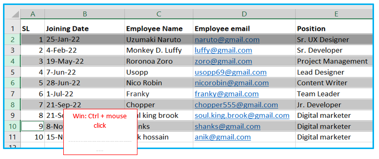
Mac: If you’re using a Mac, you may select each row by clicking on the matching number on the spreadsheet’s left side while depressing the command key on your keyboard. (Command (or Cmd) ⌘ + mouse click)
Windows: If you’re using Windows, you can click on the relevant number for each row on the left side of the spreadsheet while holding down the control key on your keyboard and using your mouse or trackpad (Ctrl + mouse click).
2. Conditional Formatting:
This technique can be used to choose alternate rows in a certain group of cells and modify the formatting. This approach is limited to Windows and is ineffective for choosing which rows to include in a calculation. You can take the following actions:
The procedure of selecting every other row using conditional formatting in Excel:
Step 1: Select the data set on your need. Now here we are selecting the all data on my spreadsheet (A1:E11 in this case)
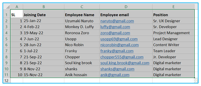
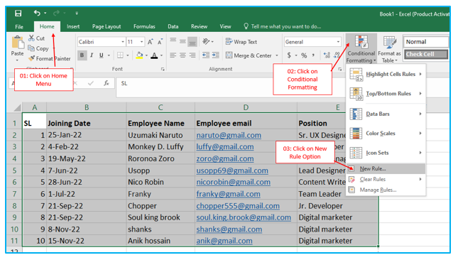
Step 2: Launch the Conditional Formatting dialog box by selecting New Rule from the Home menu (Keyboard Shortcut: Alt + O + D).
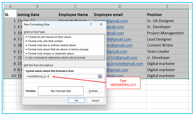
Step 3: After you click on the “New Rule” option it will show you a dialogue box like the image down below. Then click on the “Use a Formula to determine which cells to format” option.
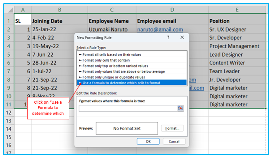
Step 4: Enter the following formula in the area under Edit the Rule Description: =MOD(ROW(),2)=1.
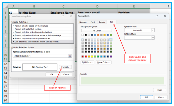
Step 5: Click on the Format button to set the formatting that you want. Now we choose to fill color here. After completing your format then click the ok button.
Step 6: Again, click the OK button.
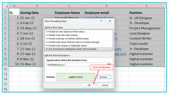
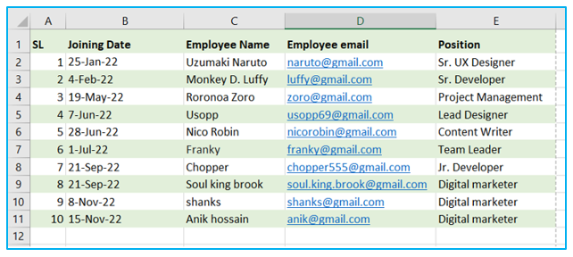
Once you’ve finished with all the dialog windows, click OK. When you return to your spreadsheet, every other row should display the format that you choose.
3. Format Data as a Table:
You can format your table using various preset formatting options in Excel. Your table may appear more structured and professional with these formats. For a better reading, a few of these pre-made table styles have alternating colors.
These procedures can be used with these formats:
Step 1: Pick the data first, and if a header is there, select it as well.
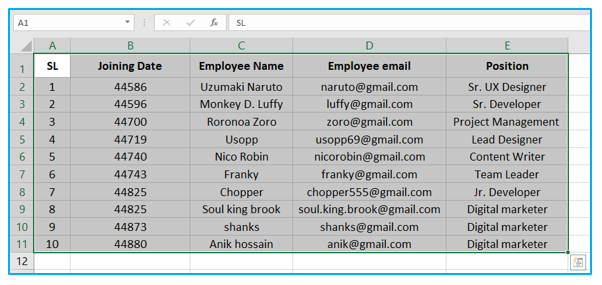
Step 2: Go to the “Insert” tab and then click the “Table” option under “Tables” section, outlined in Red below. (Keyboard Shortcut: CTRL+T).

Step 3: A dialog window labeled “Create Table” will appear. Make sure the range of cells you plan to format as a table is accurate by checking it again.
If you need to make a change, you can either click the tiny upward arrow and then use the mouse to pick the cells from your worksheet, or you can just overwrite the cell range in the box.
Make sure the “My table has headers” option is checked if your data contains headers. Select OK.
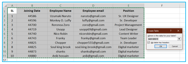
Your information will now be presented in table object format. Every other row will be colored, and the default color formatting will be used.

By choosing any cell in your data table and clicking Table Design on the ribbon, you can quickly change the color formatting.
Step 4: You can choose the table’s color from several pre-set formats in the “Table Styles” section of the “Table Design” tab. Also possible is customization.
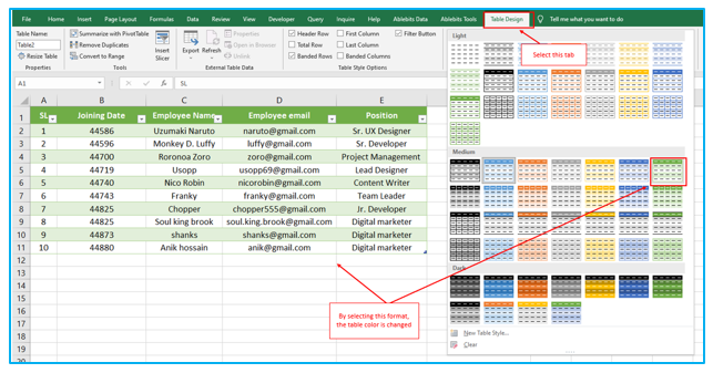
4. GO TO Special Command:
This method is excellent if you want to pick and delete every other row in your data set in Excel.
These procedures can be used with the “Go To Special” command:
Step 1: In the last column on the right side of our data set, we first add a “Helper” column. Give it a header to indicate its purpose, as it will be erased afterward.
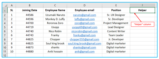
Step 2: Put an “X” in the helper column’s first row. Then, after clicking on this cell, drag the mouse down to the cell below it to select both.
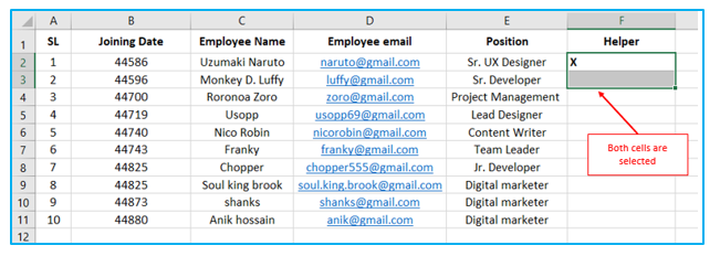
Step 3: Now that the first two cells have been selected, you may have noticed the Auto Fill Handle, a tiny green square in the bottom right corner of the selected cells.
To extend the selection to all the rows in your data set, click and hold the Auto Fill Handle while dragging the mouse downward.
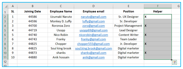
Step 4: In the helper column, we now have an identifiable pattern of “X then blank” for every two cells. Continue to choose these cells by going to the “Home” tab, clicking “Find & Select,” and then selecting “Go To Special.”

Step 5: The “Go To Special” dialog box will then be displayed. Click OK after selecting the “Blanks” radio choice.
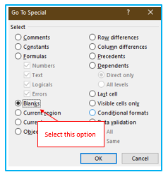
Step 6: The empty cells in the helper column will now be the subject of a non-contiguous cell selection created by Excel. Now we can select Delete with the right-click menu on any of the chosen cells.
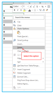
Step 7: By doing so, the “Delete” dialog box will open, allowing you to choose “Entire Row” and then click “OK.”
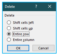
The data will be pushed up into the gaps after every other row has been deleted.

5. Using Filter:
Three ways mentioned previously assist you in formatting alternate rows for better readability. In some cases, though, formatting the rows is preferable to removing them or using them in a calculation.
These procedures can be used with the Filter option:
Step 1: Pick the data first, and if a header is there, select it as well.
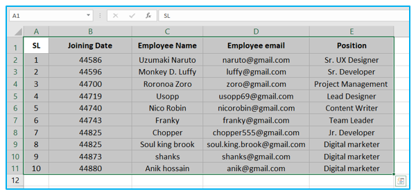
Step 2: Go to the “Insert” tab and then click the “Table” option under “Tables” section, outlined in Red below. (Keyboard Shortcut: CTRL+T).
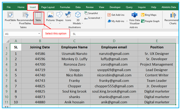
Step 3: A dialog window labeled “Create Table” will appear. Make sure the range of cells you plan to format as a table is accurate by checking it again.
If you need to make a change, you can either click the tiny upward arrow and then use the mouse to pick the cells from your worksheet, or you can just overwrite the cell range in the box.
Make sure the “My table has headers” option is checked if your data contains headers. Select OK.
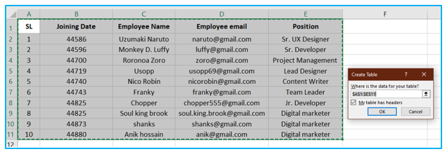
Your information will now be presented in table object format. Every other row will be colored, and the default color formatting will be used.
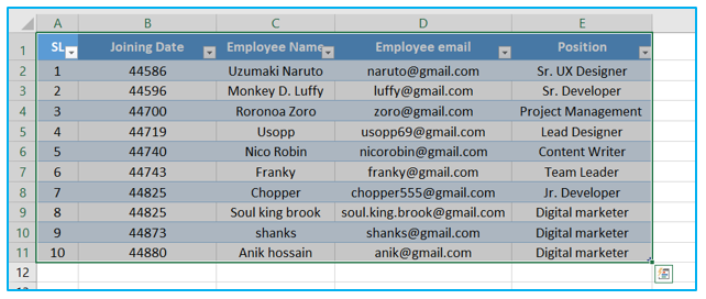
By choosing any cell in your data table and clicking Table Design on the ribbon, you can quickly change the color formatting.
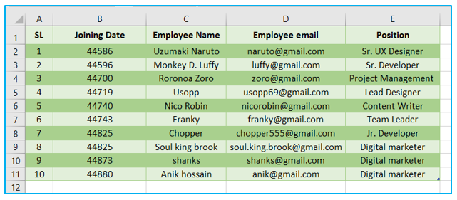
Step 4: Go to the “Home” tab, click “Sort & Filter,” and then select “Filter.”

Step 5: Drop-down menus will now display at the top of the table you’ve chosen.
Select the data you wish to filter by clicking the drop-down menu in the column (In this example, I select “Position”). As the filter impacts the entire sheet and not just the selected cells, be sure there are no other pieces of information in your sheet that could change if it is applied.
Select the option you wish to emphasize from the Filter drop-down list (In this example, I select “Digital Marketer”)
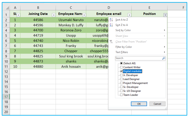
Cells are then highlighted after that. The outcome is displayed below.

Application of Every Other Row in Excel
- Data Visibility Enhancement:
- Apply alternating colors to rows for better data visibility, making it easier to distinguish individual records in large datasets.
- Facilitating Reading and Analysis:
- Improve readability in tables by using alternating row colors, allowing users to follow data patterns and analyze information more efficiently.
- Creating Data Tables:
- Enhance the visual appeal of data tables by applying every other row formatting, contributing to a well-organized and professional-looking spreadsheet.
- Highlighting Specific Information:
- Use alternating row colors to highlight specific types of information, making it visually clear and aiding in the identification of relevant data.
- Conditional Formatting Effects:
- Combine alternating row colors with conditional formatting rules to create dynamic visual effects, drawing attention to specific conditions or trends in the data.
- Printing and Report Generation:
- Improve the presentation of printed Excel sheets or reports by applying every other row formatting, resulting in a clean and structured appearance.
Utilizing Every Other Row formatting is a versatile technique that not only enhances the aesthetics of your Excel sheets but also contributes to improved data interpretation and analysis.
You may be interested:
