Highlight Active Row Column in Excel to revolutionize the way you interact with complex datasets, ensuring clarity and focus in your data analysis endeavors. This technique is invaluable for professionals dealing with extensive spreadsheets, as it instantly illuminates the active area, reducing errors and enhancing productivity. Whether you’re crunching numbers, managing large inventories, or tracking project timelines, this guide will walk you through the steps to effectively employ this visual aid, turning your Excel worksheets into a highly intuitive and user-friendly environment.
You will discover three distinct techniques in this tutorial to highlight active row column in Excel.
This Tutorial Cover:
- Automatically highlight active row column using VBA
- Customizing the code
- Adding VBA code to your worksheet
- Highlight active row and column without VBA
- Utilizing conditional formatting and VBA, highlight a particular row and column.
- How to highlight active row
- How to highlight active column
- How to highlight active row and column
1. Automatically highlight Active Row Column using VBA
This example demonstrates how to programmatically highlight an active column and row in VBA. We will make use of the Worksheet object’s SelectionChange event for this.
First, by setting the ColorIndex attribute to 0, you remove the background color from every cell on the sheet. Then, by changing the ColorIndex property of the active cell’s row and column to the chosen color’s index number, you may highlight the entire row and column.
Private Sub Worksheet_SelectionChange(ByVal Target As Range)
If Target.Cells.Count > 1 Then Exit Sub
Application.ScreenUpdating = False
‘Clear the color of all cells
Cells.Interior.ColorIndex = 0
With Target
‘Highlight row and column of the selected cell
EntireRow.Interior.ColorIndex = 42
EntireColumn.Interior.ColorIndex = 43
End With
Application.ScreenUpdating = True
End Sub
Customizing the code:
These simple suggestions might help you modify the code to suit your needs:
- The gif above shows how our sample code uses two different colors, 42 for the row and 43 for the column. Simply substitute those with any other ColorIndex codes of your own to alter the highlight color.
- Use the same color index number for both the row and the column to achieve the uniform coloring.
- This line should be deleted or commented out to simply highlight the active row: EntireColumn.Interior.ColorIndex = 43
- Remove or comment out this line to simply highlight the active column: EntireRow.Interior.ColorIndex = 42
- Adding VBA code to your worksheet:
You must place the code in the worksheet’s code window rather than the standard module if you want it to be executed silently in the background of that worksheet. Follow these instructions to get it finished:
- Press Alt + F11 in your workbook to access the VBA editor.
- You may see a list of all open workbooks and associated worksheets in the Project Explorer, which is located on the left. Use the shortcut Ctrl + R to bring up the Project Explorer window if you can’t see it.
- Locate the desired worksheet. Select the sheet you wish to highlight by double-clicking on it in the Microsoft Excel Objects folder. It is Sheet 1 in this instance.
- Paste the aforementioned code into the Code window on the right. Save the document as a Macro-Enabled Workbook (.xlsm).
Advantages: All work is done in the background; no user-side modifications or customizations are required; works with all Excel versions.
Drawbacks: There are two major drawbacks that render this technique inapplicable in some situations:
- The code removes all background colors from each spreadsheet cell. Avoid using this method if you have colorful cells since your custom formatting will be lost.
- By running this code, the sheet’s undo functionality is disabled, making it impossible to use the Ctrl + Z keyboard shortcut to reverse an error.
2. Highlight active row and column without VBA
Excel’s conditional formatting is the best you can do without VBA to highlight the selected row and/or column.
Follow these instructions to set it up:
Step 1: Choose the dataset where the highlighting is to be done.
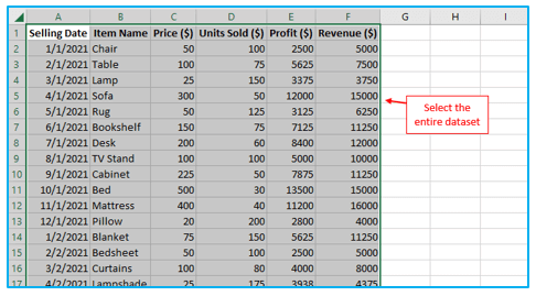
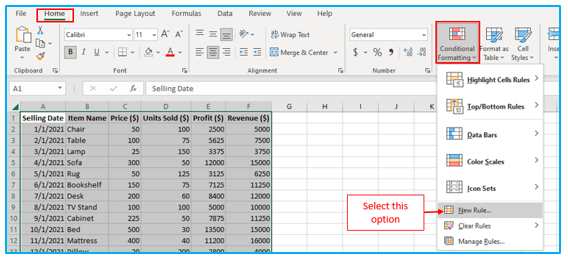
Step 2: Click “New Rule” from “Conditional Formatting” option under the “Styles” group on the “Home” tab.
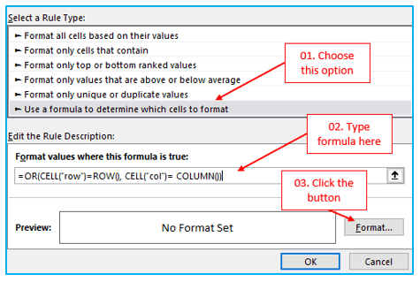
Step 3: Select “Use a formula to determine which cells to format” in the “New Formatting Rule” dialog box. Enter one of the following formulas in the Format values where this formula is true box:
- To excel highlight active row:
=CELL(“row”)=ROW()
- To highlight active column:
=CELL(“col”)=COLUMN()
- To highlight active row and column:
=OR(CELL(“row”)=ROW(), CELL(“col”)= COLUMN())
The CELL function is used in each formula to return the row/column number of the chosen cell.
For this example, we chose to highlight the column and row using the OR algorithm. That requires less effort and work in most situations.
After entering the formula, To choose a color, click the “Format” button.
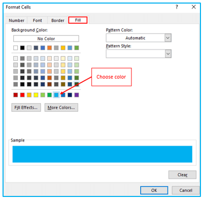
Step 4: After clicking “Format” button choose the “Fill” tab. To close both dialog windows, click OK twice.
Step 5: Unfortunately, because it necessitates manually recalculating the sheet, this approach is not as nice as the VBA one (by pressing the F9 key). By default, Excel does not recalculate a worksheet when the selection changes; instead, it does so only after adding new data or changing an old one. You choose a different cell, but nothing happens. Press F9 to update the highlighting, reload the document, and recalculate the calculation.
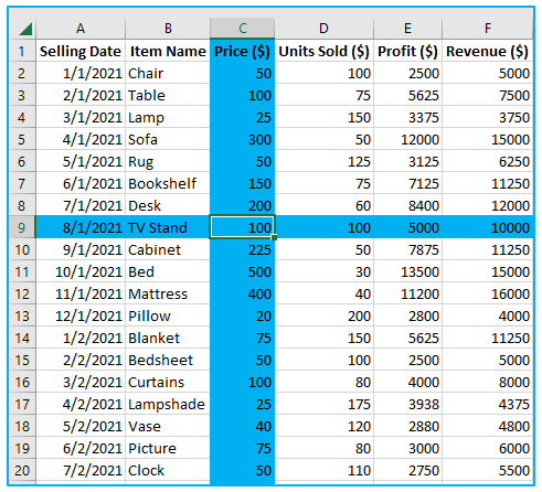
Place the following straightforward VBA code in the code module of your target sheet, as demonstrated in the previous example, to have the worksheet automatically recalculated anytime the SelectionChange event takes place:
Private Sub Worksheet_SelectionChange(ByVal Target As Range)
Target.Calculate
End Sub
The code makes the chosen range or cell recalculate, which makes the CELL function update and the conditional formatting takes the new value into account.
Pros: Unlike the previous method, this one preserves any existing formatting that you have manually added.
Cons: Could make Excel perform worse.
- The conditional formatting must be made to recalculate the formula each time a selection is changed for Excel to function (either manually with the F9 key or automatically with VBA). Forced recalculations could make Excel lag. Since our method simply recalculates the selected cells, rather than the full sheet, only really big and complicated workbooks are likely to see a detrimental impact.
- The technique won’t perform in earlier versions of Excel because the CELL function is only accessible in Excel 2007 and higher.
3. Utilizing conditional formatting and VBA, highlight a particular row and column
If the preceding approach causes your workbook to open slowly, you can try an alternative strategy: instead of recalculating a worksheet with each user movement, use VBA to acquire the current row/column number, which you can then provide to the ROW() or COLUMN() function using conditional formatting formulae.
These are the activities you must do in order to achieve this:
Step 1: Make a new blank sheet and label it Helper Sheet in your workbook. This sheet’s sole function is to securely save two numbers that represent the row and column in which a particular cell is located so that you can later safely conceal the sheet.
![]()
Step 2: Put the following VBA in the worksheet’s code window where you want to use it to implement highlighting. Please see our first example for the full instructions.
Private Sub Worksheet_SelectionChange(ByVal Target As Range)
Application.ScreenUpdating = False
Worksheets(“Helper Sheet”).Cells(2, 1) = Target.Row
Worksheets(“Helper Sheet”).Cells(2, 2) = Target.Column
Application.ScreenUpdating = True
End Sub
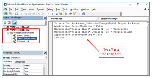
The code above adds the active row’s and column’s coordinates to the “Helper Sheet” sheet. Change the worksheet name in the code if you called your sheet differently in step 1 than you did. A2 and B2 are used to indicate the row and column numbers, respectively.
Step 3: Select the full dataset in your target worksheet, then use the formulas below to construct a conditional formatting rule. The aforementioned example gives detailed instructions.

Let’s now go into more detail about the three key use cases.
- How to highlight active row?
How to highlight row in excel by utilizing conditional formatting and VBA is shown below:
Create a conditional formatting rule with the following formula to highlight the row where your cursor is now located:
=ROW()=’Helper Sheet’!$A$2
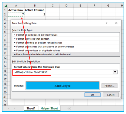
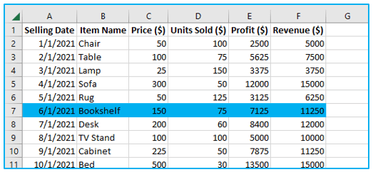
As a result, the user may see exactly which row is chosen at the moment:
- How to highlight active column?
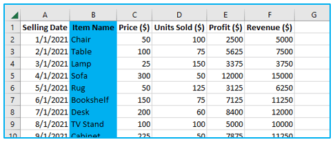
Use the following formula to pass the column number to the COLUMN function in order to highlight the chosen column:
=COLUMN()=’Helper Sheet’!$B$2
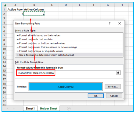
Now, you may easily and comfortably view vertical data by concentrating only on a highlighted column.
- How to highlight active row and column?
How to highlight in excel rows and columns is shown below:
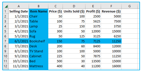
Combine the ROW() and COLUMN() methods into one formula to automatically shade the selected row and column in the same color:
=OR(ROW()=’Helper Sheet’!$A$2, COLUMN()=’Helper Sheet’!$B$2)
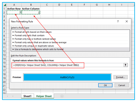
The pertinent information is brought into focus right away, helping you to avoid misinterpreting it.
Pros: enhanced performance; compatible with all Excel versions.
Cons: the prolonged setup.
That is how you highlight a chosen cell’s column and row in Excel. I appreciate you reading, and I sincerely hope this tutorial was helpful.
For ready-to-use Dashboard Templates:
