Duplicates Value in Excel refers to the presence of identical data entries within a dataset, which can often lead to inaccuracies or inefficiencies in data analysis. By identifying and removing duplicate values, users can ensure data integrity and accuracy in their spreadsheets. Excel offers various tools and functions to detect and manage duplicate values, such as Conditional Formatting, Remove Duplicates, and COUNTIF function. Removing duplicate values streamlines data analysis processes, enhances decision-making accuracy, and improves overall data quality. Utilizing these features enables users to efficiently manage and manipulate data, resulting in more reliable and meaningful insights.
This Tutorial Covers:
- How to find duplicate values in Excel
- How to identify duplicate records with 1st occurrences
- How to identify duplicate records without 1st occurrences
- How to make Excel highlight duplicates
- How to highlight duplicate records without the first occurrence
- How to search for duplicate rows in Excel
- How to calculate duplicates in Excel
- Count each occurrence of a duplicate record separately
- Determine the overall number of duplicates in a column.(s)
- How to use Excel to filter duplicates
- How to display and hide duplicates in Excel
- How to filter duplicates based on how often they appear
- How to delete duplicates from Excel
1. How to find duplicate values in Excel?
The COUNTIF function in Excel is the simplest tool for finding duplicates. The formula will differ slightly depending on whether you wish to discover duplicate values with or without initial occurrences, as demonstrated in the following instances.
-
How to identify duplicate records with 1st occurrences?
One scenario is given where you have a dataset, and you need to identify if there are any duplicate values present in column B.
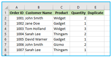
The steps to identify duplicate records with 1st occurrences are described below:
Step 1: To duplicate the formula down to other cells, enter the following formula in E2, then choose E2, then drag the fill handle:
=COUNTIF(B:B, B2)>1
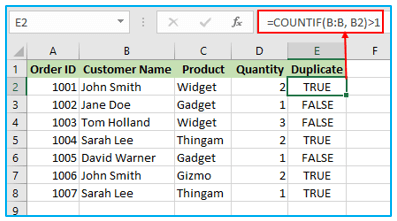
The formula returns TRUE for duplicate values and FALSE for unique values, as shown in the screenshot above.
Note: Remember to lock that range with the $ sign if you need to search for duplicates within a set of cells rather than throughout a whole column. Use this formula, for instance, to look for duplicates in cells B2 through B8:
=COUNTIF($B$2:$B$8, B2)>1
Put a duplicate formula inside the IF function and type any labels you like for duplicate and unique values to get it to produce something other than the Boolean values TRUE and FALSE:
=IF(COUNTIF($B$2:$B$8, $B2)>1, “Duplicate”, “Unique”)
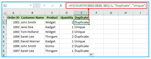
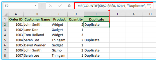
Replace “Unique” with an empty string (“”) if you want an Excel formula to just discover duplicates:
=IF(COUNTIF($B$2:$B$8, B2)>1, “Duplicate”, “”)
The formula will return “Duplicates” for records that have duplicates, and a blank cell for records that have unique records:
-
How to identify duplicate records without 1st occurrences?
Using the formula above is risky because it flags all identical entries as duplicates, which is undesirable if you intend to filter or delete duplicates after detecting them. Additionally, you can only get rid of the second and any succeeding instances of a duplicate record if you want to maintain the list’s unique values.
The steps to identify duplicate records without 1st occurrences are described below:
Step 1: To duplicate the formula down to other cells, enter the following formula in E2, then choose E2, then drag the fill handle:
=IF(COUNTIF($B$2:$B2, $B2)>1, “Duplicate”, “”)
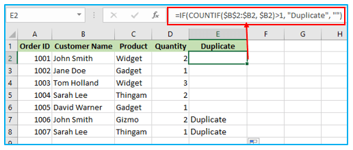
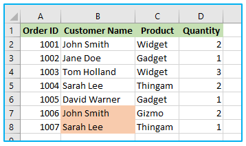
This formula does not identify the first instance of “John Smith” as a duplicate, as shown in the screenshot above.
2. How to make Excel highlight duplicates?
There is a predefined rule for highlighting duplicate cells in every version of Excel.
Follow these steps to highlight duplicate in your worksheets:
Step 1: Choose the data you prefer to examine for duplications.

Step 2: Click “Conditional Formatting” under the “Styles” category on the “Home” tab, then choose “Highlight Cells Rules,” and finally click “Duplicate Values…”
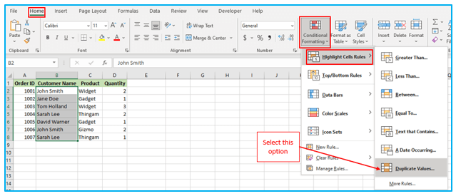
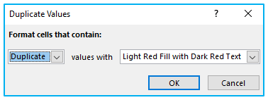
Step 3: The default settings for the “Duplicate Values” dialog window’s fill and text colors are Light Red Fill and Dark Red, respectively. Just click OK to use the default formatting.
After clicking OK, the result looks like below:
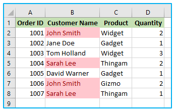
There are a few other predetermined formats in the dropdown list in addition to the red fill and text formatting. Click Custom Format… (the last option in the drop-down) and choose your preferred fill and/or font color to shade duplicates with a different color.
-
How to highlight duplicate records without the first occurrence?
Following are the procedures to emphasize the second and all subsequent duplicate occurrences:
Step 1: Choose the data you prefer to examine for duplications.
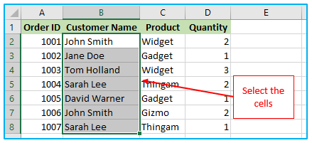
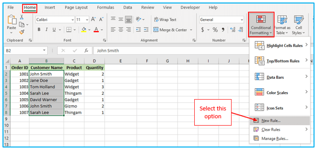
Step 2: Click “New rule” after selecting “Conditional Formatting” from the “Styles” group under the “Home” menu.
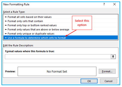
Step 3: Choose the “Use a formula to determine which cells to format” option from the “New Formatting Rule” window that has just shown.
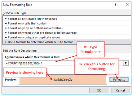
Step 4: Enter the following formula in the area marked Format values where this formula is true:
=COUNTIF($B$2:$B2,$B2)>1
Select the fill and/or font color you desire by clicking the “Format…” button.
To save and apply the rule, click OK at the very end.
The duplicate cells, with the exception of first instances, will thereafter be highlighted in the color of your choice:
3. How to search for duplicate rows in Excel?
If your goal is to dedupe a table with multiple columns, you’ll need a formula that can examine each column and only discover absolute duplicate rows, or rows with exactly the same values in every column.
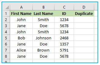
Let’s think about the following dataset.
The steps to search for duplicate rows with 1st occurrences in Excel are described below:
Step 1: To duplicate the formula down to other cells, enter the following formula in E2, then choose E2, then drag the fill handle:
=IF(COUNTIFS($A$2:$A$8,$A2,$B$2:$B$8,$B2,$C$2:$C$8,$C2)>1, “Duplicate row”, “”)

The screenshot that follows shows that the formula actually only finds rows with identical values across all three columns. For instance, row 6 is not considered a duplicate row because it includes a distinct ID in column C.
If you want to display duplicate rows without first occurrences, make the following small change to the formula:
=IF(COUNTIFS($A$2:$A2,A2, $B$2:$B2,B2,$C$2:$C2,C2) >1, “Duplicate row”, “”)

4. How to calculate duplicates in Excel?
To determine the precise number of identical records present in your Excel spreadsheet, you can utilize one of the formulas provided below to count the occurrences of duplicates.
-
Count each occurrence of a duplicate record separately:
You may frequently need to know how many duplicates there are for each value in a column of duplicated data.
Use the COUNTIF formula to calculate the frequency of each element in your Excel worksheet.
The steps to count each occurrence of a duplicate record separately are described below:
Step 1: To duplicate the formula down to other cells, enter the following formula in C2, then choose C2, then drag the fill handle:
=COUNTIF($A$2:$A$9, $A2)

As demonstrated in the above screenshot, the formula counts the occurrences of each name: “John ” occurs 3 times, “Jane ” – 2 times, “Michael ” . “Samantha ” and “Emily ” only once.
Use the following formula to determine the first, second, third, etc. occurrences of each item:
=COUNTIF($A$2:$A2, $A2)
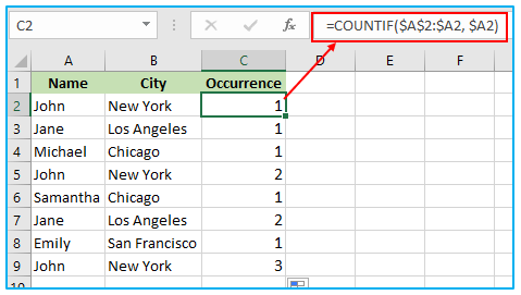
You can also count the instances of duplicate rows in a similar way. The main difference is that COUNTIF will no longer work; you must use COUNTIFS instead.
=COUNTIFS($A$2:$A$9, $A2, $B$2:$B$9, $B2)
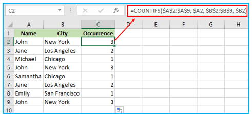
You can hide unique values and only see duplicates after the duplicate values have been counted, or you can do the opposite. Apply Excel’s auto-filter to achieve this.
-
Determine the overall number of duplicates in a column.(s):
Using any of the formulae we used to find duplicates in Excel (with or without first occurrences) is the simplest approach to count duplicates in a column. Using the COUNTIF algorithm below, you can then determine the number of duplicate values:
=COUNTIF(range, “duplicate”)
Where “duplicate” is the term you used in the duplicate-finding formula.
In this illustration, our duplication formula looks like this:
=COUNTIF(C2:C9, “Duplicate”)
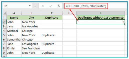
Use a more complicated array formula to count duplicate values in Excel. This method has the benefit of not requiring a helper column:
=ROWS($A$2:$A$9)-SUM(IF( COUNTIF($A$2:$A$9,$A$2:$A$9)=1,1,0))
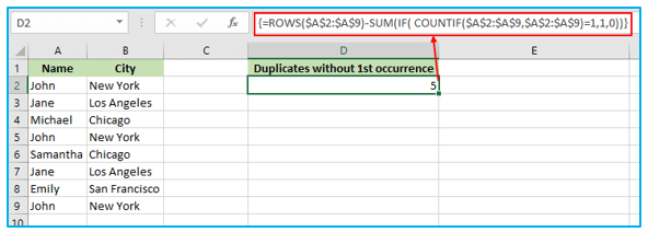
Note: Remember to enter the formula by pressing Ctrl + Shift + Enter because it is an array formula. Please be aware that this calculation includes initial occurrences when counting duplicate records.
To determine the count of duplicate rows in a dataset, replace the COUNTIF function with the COUNTIFS function and include the columns that need to be checked for duplicates in the formula.
=ROWS($A$2:$A$9)-SUM(IF( COUNTIFS($A$2:$A$9,$A$2:$A$9, $B$2:$B$9,$B$2:$B$9)=1,1,0))

5. How to use Excel to filter duplicates?
If you want to simplify your data analysis, you can apply filters to display only duplicate records. Alternatively, if you need to focus on unique entries, you can hide the duplicates and view only the distinct records. Here are solutions for both situations.
-
How to display and hide duplicates in Excel?
To easily identify all duplicates in your Excel table, choose an appropriate formula from the available options.
The steps to display and hide duplicates in Excel are described below:
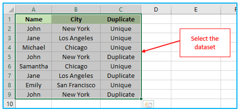
Step 1: Select the dataset.
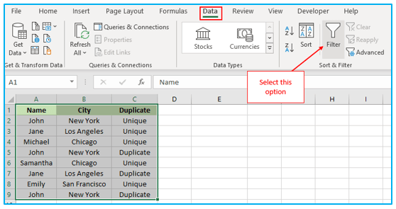
Step 2: Go to the “Data” tab and click on the “Filter” button.
Another option is to go to the “Home” tab, select “Sort & Filter”, and then click on “Filter” in the “Editing” group.
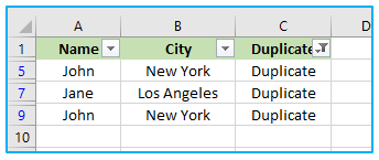
Step 3: Next, click on the filtering arrow located in the header of the Duplicate column, and mark the checkbox for “Duplicate” to display all duplicates. Select OK.
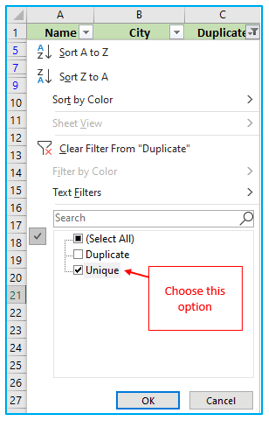
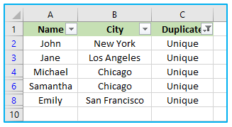
Conversely, to hide the duplicates, select “Unique” to view only the unique records.
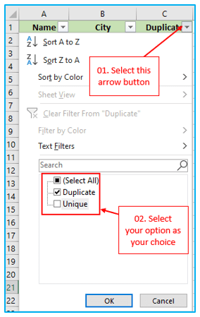
The result looks like below:
Conversely, to hide the duplicates, select “Unique” to view only the unique records.
The result looks like below:
Note: A helpful tip to activate filtering automatically is to transform your data into a fully functional Excel table. To do this, highlight all the data and use the Ctrl + T keyboard shortcut.
-
How to filter duplicates based on how often they appear?
If you want to view the 2nd, 3rd, or any specific instance of duplicate values, you can use the formula mentioned earlier to count the occurrences of duplicates.
Once you have applied the formula, filter your table, and choose the particular occurrence(s) you wish to view. For instance, to display the 3rd occurrence, you can apply a filter as shown in the provided screenshot.

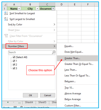
Click the filter arrow in the header of the “Occurrences” column (the formula column) and then select Number Filters > Greater Than to display all duplicate data, that is, occurrences greater than 1.
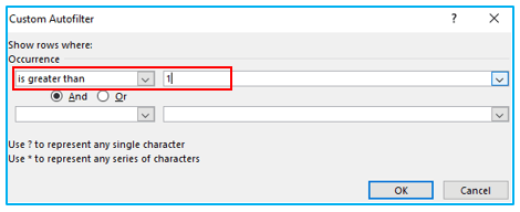
Click the OK button after selecting “is greater than” in the first box and entering 1 in the box next to it:
The result looks like below:
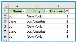
Similarly, you can display the 2nd, 3rd, or any subsequent duplicate occurrence by typing the desired number in the box next to “is greater than”.
-
How to delete duplicates from Excel?
Excel duplicates can be removed by selecting them, doing a right-click, and selecting “Clear Contents” (or by selecting Clear > Clear Contents from the Home tab’s Editing group). You will end up with empty cells because this will just erase the contents of the cells. The same result can be obtained by selecting the filtered duplicate cells and pressing the Delete key.
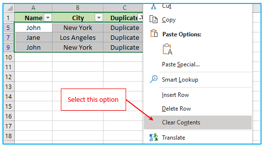
Filter duplicate rows, drag the mouse over the row headings to pick the rows, right-click the selection, and then select “Delete Row” from the context menu.

Application of Duplicates Value in Excel
- Data Cleaning: Identifying and removing duplicate values is crucial for cleaning datasets, ensuring data accuracy, and maintaining integrity.
- Data Validation: Detecting duplicates helps in validating data input, preventing errors, and maintaining consistency in datasets.
- Data Analysis: Eliminating duplicates before analysis ensures that each data point is considered only once, leading to accurate insights.
- Conditional Formatting: Applying conditional formatting to highlight duplicate values visually aids in quick identification and analysis.
- Database Management: Removing duplicate entries in databases improves efficiency and prevents redundancy in data storage.
- Error Prevention: Eliminating duplicate values reduces the risk of errors in calculations, summaries, and reports based on the data.
For ready-to-use Dashboard Templates:
