Picture Lookup in Excel is a game-changer for visual data retrieval, allowing you to associate images with specific data entries for enhanced understanding and analysis. By incorporating pictures into your lookup tables, you can easily identify and reference information based on visual cues. Say goodbye to traditional text-based lookups and hello to a more intuitive and efficient way of working with your data. Whether you’re creating product catalogs, inventory management systems, or educational materials, Picture Lookup in Excel offers endless possibilities for improving data comprehension and presentation. Embrace this innovative feature to elevate your Excel experience and unlock new levels of insight and creativity in your spreadsheets. With Picture Lookup, you can transform your data into a visually engaging and informative resource that brings your information to life.
This Tutorial Covers:
- Picture Lookup – Introduction
- Some benefits of Picture Lookup
- How to create a picture lookup
- Getting the data set ready
- Creating a drop-down list to show item names
- Creating a Linked Picture
- Creating a Named Range
1. Picture Lookup – Introduction
The Excel lookup functions VLOOKUP, LOOKUP, and XLOOKUP, among others, can be used to look up data from a list. Additionally, it is a given that a list of photos cannot be returned by these lookup functions. The adage “One image is worth a thousand words” is well known.
Since an Excel Picture Lookup displays visuals, it will make the data more interesting to viewers.
Numerous uses for this feature include sales, small businesses, company units, etc. It is advised that any company that needs data, including photographs, use this capability.
2. Some benefits of Picture Lookup
- Improved data accuracy.
- Attractive and simple to understand.
- Accurate designation of the subject.
- Authenticating companies.
3. How to create a picture lookup
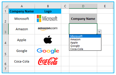
I’ve got a list of five companies name, and their logo is in the cell next to it.
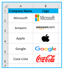
The logo of the selected team should appear when I choose a team name from the drop-down menu, which is what I want to be able to do.
This Excel picture lookup requires the following four steps to complete:
- Getting the data set ready
- Creating a drop-down list to show item names
- Creating a Linked Picture
- Creating a Named Range
Now let’s go through each of these processes in more depth.
-
Getting the data set ready
- Create a column with the names of all the objects (team names).
- Insert the item’s image in the adjacent column (club logo in this example).
Ensure that the logos fit comfortably inside the cell. You can either extend the cells or adjust the photos so that they fit inside the cell.
-
Creating a drop-down list to show item names
The steps to create a drop-down list to show item names are described below:
Step 1: Choose the cell where you want the drop-down to appear (D3 in this example).
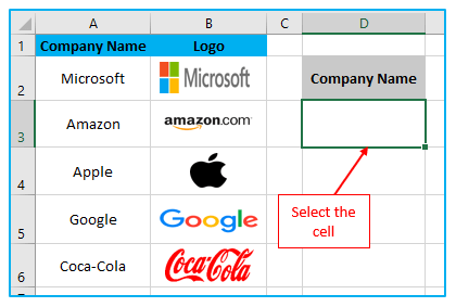
Step 2: On the “Data” tab, click. Select the “Data Validation” option by clicking on the “Data Tools” tab.

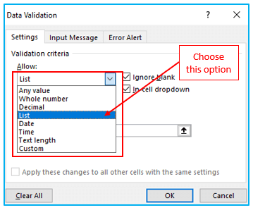
Step 3: Make sure List is selected in the Allow drop-down in the Settings tab of the Data Validation dialog box (if not selected already).
Step 4: Select the upward-pointing arrow icon in the Source field. You will be able to choose the cells where the dropdown list is contained in this way. Choose the cell range that contains the company names. Press Enter. Select OK.
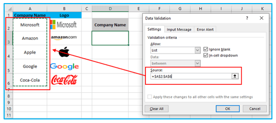
With the aforementioned actions, cell D3 would display a drop-down menu.
-
Creating a Linked Picture:
In this section, we use any of the already-existing photos or logos to generate a connected image in excel.
The stages to creating a linked picture are as follows:
Step 1: Choose a cell that contains the logo. Make sure the cell is the one you’ve chosen, not the logo or image. Copy the cell (Control + C or copy from the context menu when right-clicking).
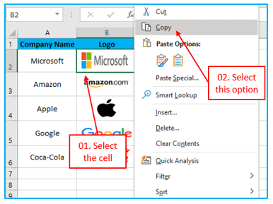
Step 2: Simply perform a right-click on the cell to obtain the related image (it can be any cell as we can adjust this later). To access more options, select Paste Special and click the tiny right-pointing arrow. Select the icon for Paste Linked Picture.
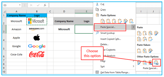
You would receive a connected image of the duplicated cell if you followed the preceding instructions. As a result, any changes you make to the copied cell will also be mirrored in the connected image.
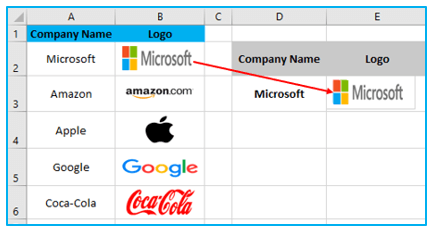
Since I cloned cell B2 in the previous image and placed a linked image there, Please take note that at this time, this is not related to the drop down.
Additionally, an image is produced when you paste the referenced image. It can therefore be moved to any location on the spreadsheet.
-
Creating a Named Range
Now that everything is set up, the final step is to ensure that the connected image changes as the selection alters. The attached image is currently only connected to one cell.
We can use a named range to link it to the drop-down menu.
The steps are as follows:
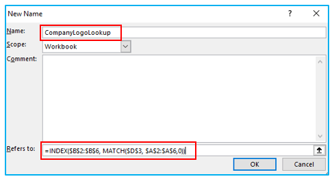
Step 1: Activate the “Formulas” tab. Select “Define Name” from the menu. The “New Name” dialog box will then be displayed.

Step 2: Make these entries in the New Name dialog box:
- Name: CompanyLogoLookup
Refers to: =INDEX($B$2:$B$6,MATCH($D$3,$A$2:$A$6,0))
After entering, click OK.
Step 3: Choose the link we made for the linked image in the previous step. The formula bar will display a cell reference, such as =$B$2. Remove the reference to this cell, then enter =CompanyLogoLookup.
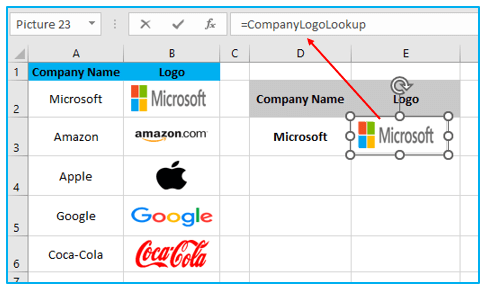
It’s done! Change the club name in the drop-down menu, and the picture will adjust accordingly.
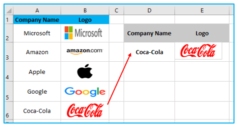
What is the process behind this picture lookup method?
The original cell from which it was cloned was referred to when we built a connected picture. With the named range, we modified that reference.
When we alter the option in the drop-down, this named range responds by returning the reference to the cell that contains the name of the selected company. For instance, if I select Coca-Cola, B6 is returned, and if I select Apple, B4 is returned.
Since we changed the reference to =CompanyLogoLookup and set the named range to the linked image, it now refers to the new cell references and thus provides an image of that cell.
The defined name must only yield a cell reference for this technique to function. The combination of the INDEX and MATCH functions is used to achieve this.
The formula is as follows:
=INDEX($B$2:$B$6,MATCH($D$3,$A$2:$A$6,0))
The location of the firm name in the drop-down list is returned by the formula’s MATCH portion. For instance, the MATCH formula would return 1 if it were Microsoft and 4 if it were Google. The INDEX function finds the reference to the cell that contains the logo (based on the position returned by MATCH).
Application of Picture Lookup in Excel
- Product Catalogs: Enhance product catalogs by associating product names or codes with corresponding images, improving visual identification and customer experience.
- Inventory Management: Improve inventory tracking by displaying product images alongside item descriptions, facilitating accurate identification and management of stock items.
- Educational Materials: Enrich educational materials, such as flashcards or study guides, by incorporating images alongside text to aid learning and retention.
- Employee Directories: Create visually engaging employee directories by including staff photos alongside names and contact information, improving recognition and team communication.
- Recipe Books: Enhance recipe books or cooking guides with images of finished dishes, allowing users to quickly identify recipes and visualize the end result.
- Training Manuals: Improve training manuals or instructional guides by including images of tools, equipment, or procedures, aiding comprehension and reducing errors.
For ready-to-use Dashboard Templates:
