Delete Rows Based on Cell Value in Excel to maintain clean, relevant, and accurate datasets for your analyses. This efficient method helps streamline data management tasks, allowing you to focus on meaningful information that drives decision-making. By mastering this technique, you can automate the process of filtering out unnecessary or erroneous data, enhancing your productivity and ensuring your Excel projects remain organized and impactful. Embrace this functionality to optimize your data processing workflows and elevate the clarity and precision of your reports.
I’ll demonstrate various methods for deleting rows in Excel based on a column value or a condition in this tutorial.
This Tutorial Covers:
- Using a value or condition, filter the rows, and then delete them
- Delete Rows that contain a specific text
- Delete Rows Based on a Numeric Condition
- After sorting the dataset, delete the rows
- Find and select the cells based on cell value, then delete the rows
- Delete every row that has a blank cell
- Delete cell based on conditional formatting
- Based on cell value, filter and delete rows (using VBA)
1. Using a value or condition, filter the rows, and then delete them
Filtering these is one of the quickest ways to remove rows that have a particular value or satisfy a certain condition. You can remove all of these rows once you have the filtered data (while the remaining rows remain intact).
With Excel’s filter, you can choose to filter based on a variety of factors (such as text, numbers, dates, and colors)
Let’s look at two instances of filtering and deleting rows.
-
Delete Rows that contain a specific text
Let’s say you wish to remove every row in the data set below where the buyer is American Eagle (in Column C).
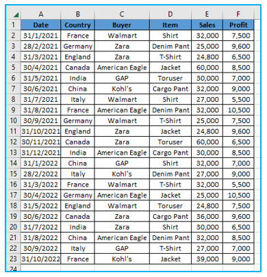
Although you can choose to manually delete these rows in this small dataset, your datasets are likely to be very large and this won’t always be an option.
Then you can delete all of these rows by filtering all the entries where American Eagle is the buyer (while keeping the other rows intact).
The steps to delete rows based on the value (all records for American Eagle) are as follows
Step 1: If you wish to remove the rows from the data set, choose any cell.
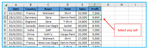
Step 2: On the “Data” tab, click. Choose the “Filter” icon under the “Sort & Filter” group. All of the dataset’s header cells will have filters applied as a result.

Step 3: The Buyer header cell’s Filter icon should be clicked (this is a small downward-pointing triangle icon at the top-right of the cell)
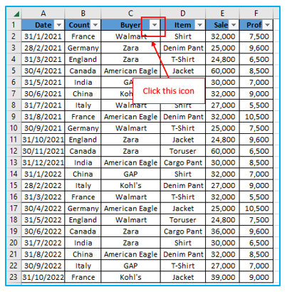
Step 4: Select the “American Eagle” choice only and deselect everything else (a quick way to do this is by clicking on the Select All option and then clicking on the American Eagle option). By applying this filter to the dataset, you will only see records for buyers of “American Eagle”. Select all the filtered records.
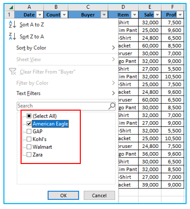
Step 5: Select “Delete Row” by selecting Right-click on any of the chosen cells.
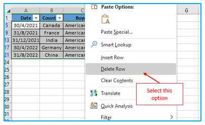
Step 6: Click OK in the dialog box that appears. You won’t find any records in the dataset at this time.

Step 7: Select the “Filter” icon from the “Data” tab. Apart from the deleted records, all records will be visible after the filter is removed.
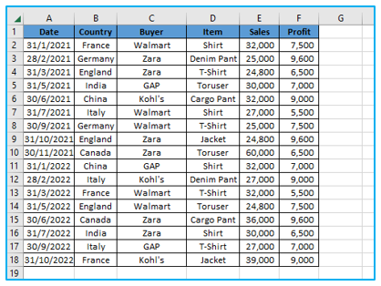
In the preceding phases, the data is first filtered based on a cell value (or other criteria like after/before a date or greater/less than a number). You simply remove the records after you have them.
Some helpful shortcuts to be aware of to quicken the process:
- To apply or remove the filter, press Control + Shift + L.
- To erase the chosen cells or rows, press Control + – (while holding down the Control key, press the minus key).
Keep in mind that everything you may have in other cells inside these rows will be lost if you delete a row. Making a copy of the data in another worksheet and deleting the rows there is one technique to get around this. Once finished, replace the original data with a copy of it.
Or
The techniques demonstrated later in this article can be used (using the Sort method or the Find All Method).
-
Delete Rows Based on a Numeric Condition
You can use a number condition (or a date condition) in the same way that I used the filter method to remove all the rows that had the text “American Eagle”.
Consider the following dataset as an example. I want to remove all the rows where the sale value is less than 30,000 from it.
The steps to delete rows based on the numeric condition are as follows
Step 1: Pick any data cell from the list.
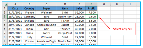
Step 2: On the “Data” tab, click. Choose the “Filter” icon under the “Sort & Filter” group. All of the dataset’s header cells will have filters applied as a result.

Step 3: In the Sales header cell, select the Filter icon (this is a small downward-pointing triangle icon at the top-right of the cell).
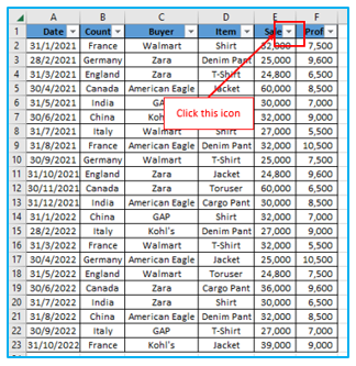
Step 4: Place your cursor on the “Number Filters” menu item. This will display all of Excel’s number-related filter choices. Select the “Less than” option by clicking.
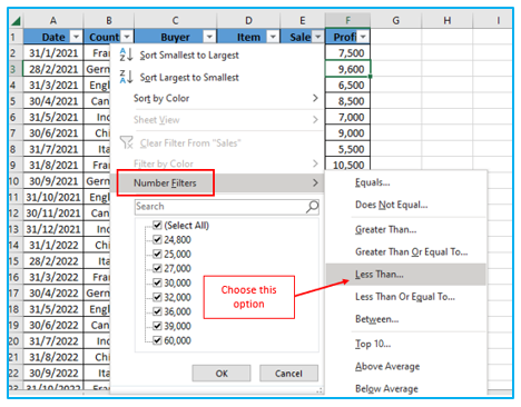
Step 5: Put “30000” in the field of the ‘Custom Autofilter’ dialog box that appears. Select OK. With this filter, only records with sales values less 30,000 will be displayed.
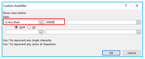
Step 6: Choose every filtered record. “Delete Row” can be selected by doing a right-click on any cell.
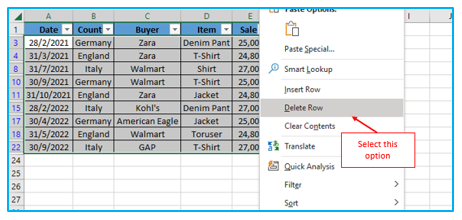
Step 7: Click OK in the dialog box that appears. You won’t find any records in the dataset at this time.
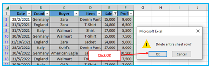
Step 8: Select the “Filter” icon from the “Data” tab. With the exception of the deleted records, all records will be visible after the filter is removed.
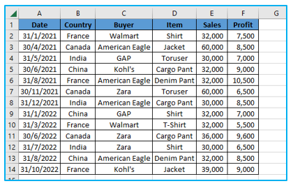
In Excel, you may apply a variety of number filters, including less than/greater than, equal/does not equal, between, top 10, above, or below average, and more.
Note: Additional filters may be used. You might eliminate all the rows where the sales value is higher than 30000 but lower than 30000, for instance. You must apply two filter conditions in this situation. Having two filter criteria is possible using the “Custom Autofilter” dialog box (AND as well as OR).
You may also filter the records depending on the date, just like you can with the number filters. For instance, by following the identical procedures as above, you can delete every record from the first quarter. Excel automatically displays pertinent filters when you are using Date filters (as shown below).
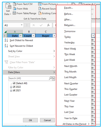
Filtering, while a terrific approach to swiftly remove rows based on a value or a condition, has one drawback: it eliminates the entire row. For instance, in the scenario below, all the data that is to the right of the filtered dataset would be deleted.
What if I only want to remove records from the dataset while retaining all of the other data?
Filtering does not allow you to accomplish that, but sorting does.
2. After sorting the dataset, delete the rows
In most situations, you’re better off utilizing the filter method described above than sorting, which is another option to delete rows depending on value.
Only when you only want to eliminate the cells with values and not the complete rows are you advised to use this sorting method.
Imagine you want to remove every record where the country is Germany from the dataset as it is displayed below.
How to accomplish this using sorting is detailed below
Step 1: Pick any data cell from the list.
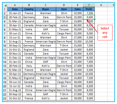
Step 2: On the Data tab, click. Simply select the “Sort” icon from the “Sort & Filter” group.

Step 3: Select “Country” in the sort by column of the Sort dialog box that appears. Check to verify that Cell Values is chosen in the Sort on field. Choose A to Z (or Z to A, it doesn’t really matter) under the Order option.
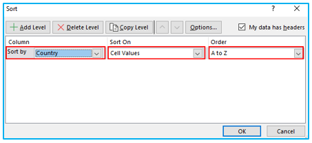
Step 4: Select OK. You will then receive the sorted data set as displayed below (sorted by column B).
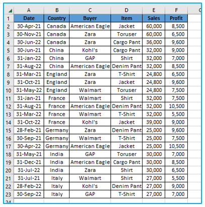
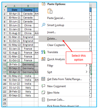
Step 5: All Germany-related records should be chosen (all the cells in the rows, not just the country column). Right-click the item you’ve chosen and then select Delete.
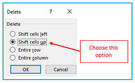
Step 6: The “Delete” dialog box will then appear. Ascertain that the ‘Shift cells up’ option is chosen. Then click OK.
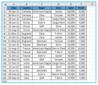
The aforementioned actions would eliminate all records with the Germany country, but they do not eliminate the entire row. Therefore, any data that is to the right or left of your dataset will be unaffected.
Although I sorted the data based on the cell value in the example above, you can also use the same methods to sort the data based on numbers, dates, the color of the cell or the color of the font, etc.
You need a means to sort the data back into the original order in the event that you wish to maintain the original data set order but eliminate records based on criteria. To accomplish this, sort the data first, then add a column with serial numbers. After you’ve finished removing the rows and records, just sort the data using the newly added column.
3. Find and select the cells based on cell value, then delete the rows
When you want to locate and pick cells with a certain value, Excel’s Find and Replace capability can be quite helpful.
You can quickly erase the rows after selecting these cells.
Let’s say you have the dataset depicted below and wish to remove every row where Germany is listed as the country.
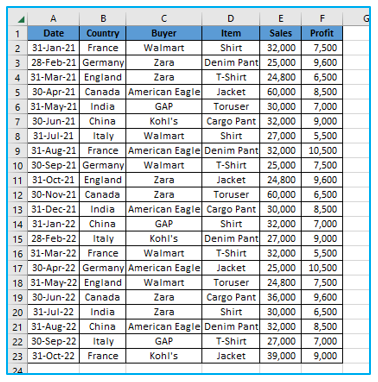
The procedures are as follows:
Step 1: Choose the whole set of data.

Step 2: On the “Home” tab, click. Select the “Find & Select” option under the “Editing” group, and then click “Find” (you may alternatively use the keyboard shortcut Control + F).
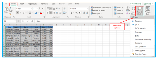
Step 3: In the “Find what:” field of the Find and Replace dialog box, type “Germany”. Select “Find All”. This will display all occurrences of the text “Germany” that Excel was able to locate for you right away. “Control + A” on the keyboard will select every cell that Excel has located. Additionally, you will be able to view every single selected cell in the dataset.
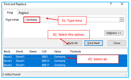
Step 4: Select “Delete” from the context menu when you right-click on any chosen cell. The “Delete” dialog box will then be displayed.
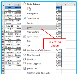
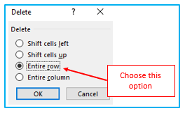
Step 5: Choose “Entire row” from the menu. Select OK.
The aforementioned actions would remove Germany from every cell.
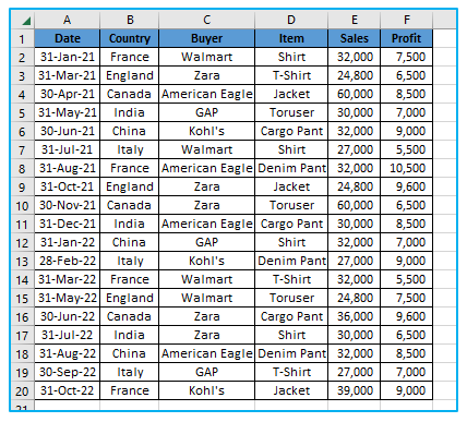
Note: You can use wildcard characters to find data in Excel because Find and Replace can handle them. Use ‘*West’ as the text to find in the Find and Replace dialog box, for instance, if you wish to remove all rows where the region is either Mid-West or South-West. This will show you every cell where the word “West” appears at the conclusion of the text.
4. Delete every row that has a blank cell
If you want to remove all the rows with blank cells, you may accomplish so quickly and effectively in Excel using a built-in feature.
You can rapidly choose all the empty cells by using the Go-To Special Cells option. Additionally, it’s really easy to delete these cells once you’ve picked all of the empty ones.
Consider the following dataset: I want to remove all the entries for which I don’t have the profit value.
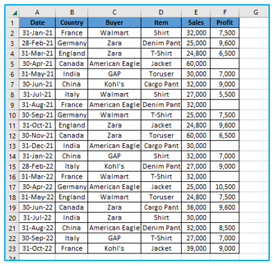
The procedures are as follows:
Step 1: Choose the whole set of data.
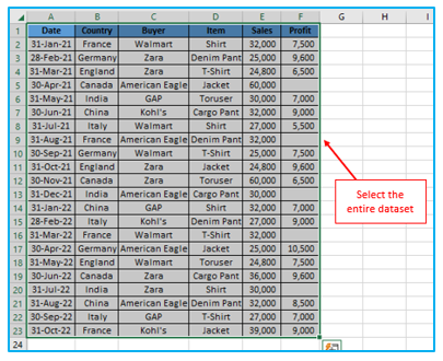
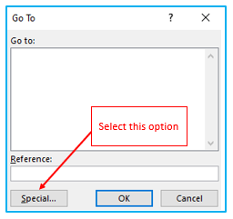
Step 2: F5 must be pressed on your keyboard. The “Go To” dialog box will then appear (you may also get it from Home -> Editing -> Find and Select -> Go To). Choose the Special button in the “Go To” dialog box. The “Go To Special” dialog box will then be displayed.
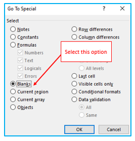
Step 3: Choose “Blanks” from the Go To Special dialog box. Select OK.
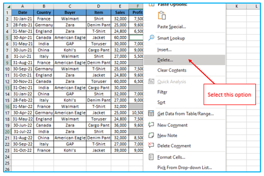
Step 4: The aforementioned actions would choose every cell in the dataset that is empty. Once the blank cells are selected, use the right-click menu to pick “Delete” from any cell.
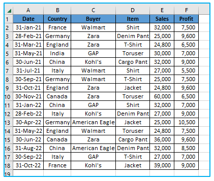
Step 5: Select “Entire row” from the drop-down menu in the Delete dialog box, then click OK

The aforementioned actions would remove blank cells.
5. Delete cell based on conditional formatting
The steps listed below should be followed if you wish to delete cells in Excel depending on conditional formatting.
Step 1: Choose the whole set of data.
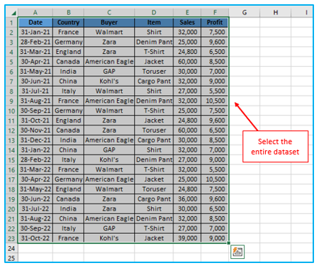
Step 2: Go to “Home” tab, then click “Conditional Formatting” option under “Styles” group. Then click “Highlight Cells Rules”, then select “Text that Contains…”.
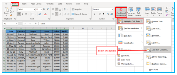
Step 3: After that, “Text That Contains” dialog box will open. In “Format cells that contain the text” box, type “American Eagle” as we want to delete this buyer’s info. Then click OK.

Step 4: On the Data tab, click. Simply select the “Sort” icon from the “Sort & Filter” group.

Step 5: Select “Buyer” in the sort by column of the Sort dialog box that appears. Check to verify that “Cell Color” is chosen in the “Sort on” field. Choose color under the “Order” option.
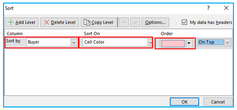
Step 6: Select OK. You will then receive the sorted data set as displayed below (sorted by column C).
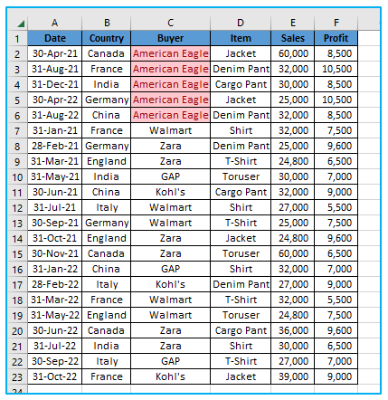
Step 7: All American Eagle-related records should be chosen (all the cells in the rows, not just the Buyer column). Right-click the item you’ve chosen and then select Delete.
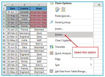
Step 8: The “Delete” dialog box will then appear. Ascertain that the ‘Shift cells up’ option is chosen. Then click OK.
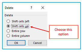
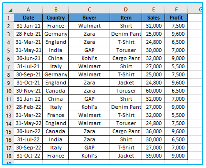
The aforementioned actions would eliminate all records with the American Eagle buyer, but they do not eliminate the entire row. Therefore, any data that is to the right or left of your dataset will be unaffected.
6. Based on cell value, filter and delete rows (using VBA)
The final technique I’ll demonstrate to you uses a small amount of VBA.
If you frequently need to delete rows based on a particular value in a column, you can use this technique. The VBA code can be added once to your Personal Macro workbook. In this manner, you can utilize it across all of your Excel workbooks.
The Filter technique described above is how this code operates (except the fact that this does all the steps in the backend and save you some clicks).
Let’s say you have the dataset depicted below and wish to remove every row where Germany is listed as the country.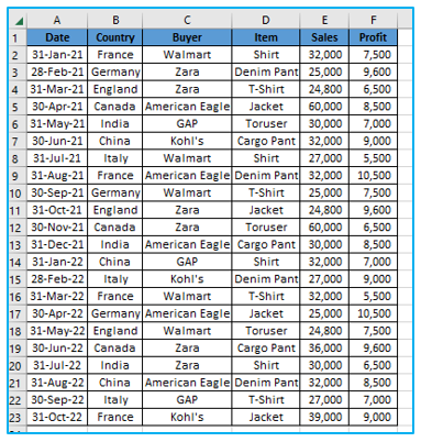
The VBA code needed for this is provided below:
Sub DeleteRowsWithSpecificText()
ActiveCell.AutoFilter Field:=2, Criteria1:=”Germany”
ActiveSheet.AutoFilter.Range.Offset(1, 0).Rows.SpecialCells(xlCellTypeVisible).Delete
End Sub
The code above first filters the rows using the supplied criteria (in this case, “Germany”), then selects all the filtered rows and deletes them.
To ensure that my header row is not erased, you’ll notice that Offset was utilized in the code above.
If your data is in an Excel Table, the code above won’t work. Excel views an Excel Table as a list object, which explains why. Thus, you must slightly adjust the code if you wish to delete rows from a Table (covered later in this tutorial).
It will present you with a prompt like seen below just before deleting the rows. This is advantageous to me because it enables me to confirm the filtered row before deleting it.

Keep in mind that you cannot revert the deletion of rows made using VBA. Use this only if you are certain that it will accomplish your goals. Additionally, keeping a backup copy of the data is a good idea in case something goes wrong.
If your data is in an Excel table, you can delete rows that have a particular value by using the code below:
Sub DeleteRowsinTables()
Dim Tbl As ListObject
Set Tbl = ActiveSheet.ListObjects(1)
ActiveCell.AutoFilter Field:=2, Criteria1:=”Germany”
Tbl.DataBodyRange.SpecialCells(xlCellTypeVisible).Delete
End Sub
I had to modify the code since VBA views Excel Table as a List object (and not a range).
Where Should the VBA Code Go?
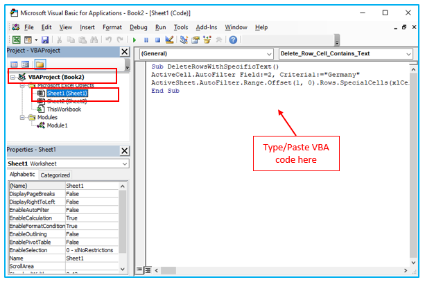
This code needs to be added to a module in the VB Editor backend.
The steps that will demonstrate how to do this are as follows:
Step 1: The VBA Editor window can be opened by pressing the keyboard shortcut ALT + F11. A “Project Explorer” pane is located in the left side of this VBA Editor window (which lists all the workbooks and worksheets objects). To use this code, double-click any object in the workbook, this will open the Module code window on the right and add the Module object to the Workbook. Copy the aforementioned code, then paste it in the module window (which will show up on the right).
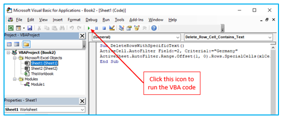
Step 2: Once the code is in the VB Editor, you can execute it using any of the following techniques (be sure to choose any cell in the dataset you wish to execute the code on first):
- Press the F5 key while selecting any line of the code.
- In the VB Editor’s toolbar, select the Run button.
- By clicking on the macro’s assigned button or form within the worksheet, you can activate it.
- Add it to the Quick Access Toolbar to instantly execute the code.
Step 3: After that, it will present you with a prompt like seen below just before deleting the rows. Click OK.

Step 4: Then, on the “Data” tab, click. Choose the “Filter” icon under the “Sort & Filter” group.

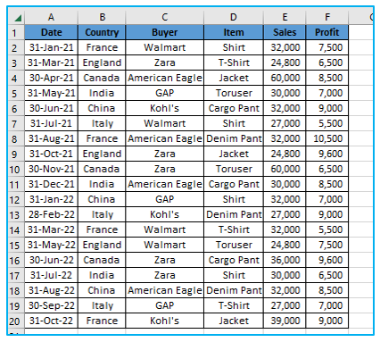
After that, the result looks like this below.
Note: You must save the workbook in the macro-enabled format because it contains VBA macro code (xlsm).
Application of Delete Rows Based on Cell Value in Excel
- Data Cleansing: Remove rows containing errors or irrelevant values, such as “#N/A” or “Error”, to clean your dataset and improve analysis accuracy.
- Filtering Out Inactive Records: Automatically delete rows that contain specific identifiers for inactive accounts, clients, or products, keeping your databases current.
- Removing Duplicate Entries: Delete rows that contain duplicate data based on specific cell values to ensure data uniqueness and integrity.
- Excluding Low-Performance Data: Automatically remove rows with performance indicators below a certain threshold, focusing analysis on higher-performing segments or individuals.
- Managing Inventory Levels: Delete rows containing products with zero inventory to streamline inventory management and reporting.
- Data Segregation: Remove rows that pertain to a specific department, geographic location, or category that is irrelevant to the current analysis or report.
For ready-to-use Dashboard Templates:
