Pivot Tables in Excel
Pivot tables are a type of table in Excel that allow you to easily summarize data. Typically, you would use a pivot table to summarize data from a large data set. The data is divided into rows and columns, and the pivot table allows you to summarize the data by different criteria. For example, you could summarize sales data by product, by region, or by month.
How do I create a pivot table ?
To create a pivot table excel, you first need to have some data in Excel that is divided into rows and columns. Once you have the data set up, go to the Insert tab and select Pivot Table.
A new worksheet will open with a blank pivot table. Drag and drop the fields from your data set into the appropriate places in the pivot table.
We use following sample table from a large data set to summarize in a pivot table:
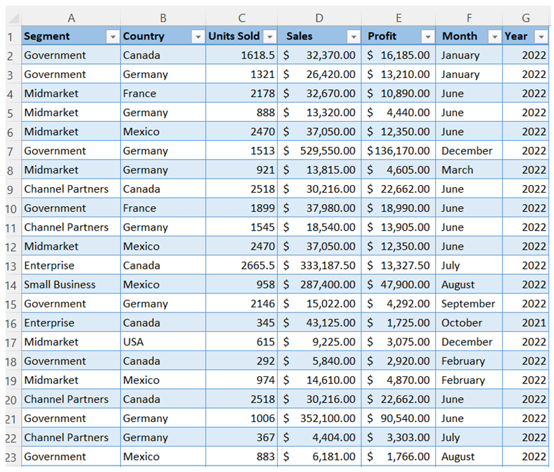
The table has 7 columns with sales and profit data in different segments and in different countries for two years splitting into months. Let’s see the process of creating the pivot table from very first stage.
How pivot table in excel inserted?
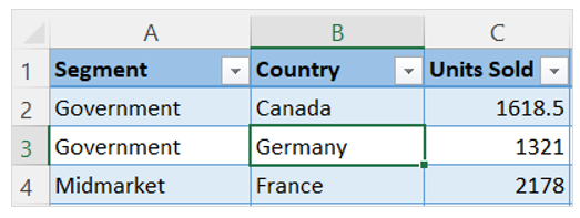
To create a pivot table, keep your cursor in any cell of data.
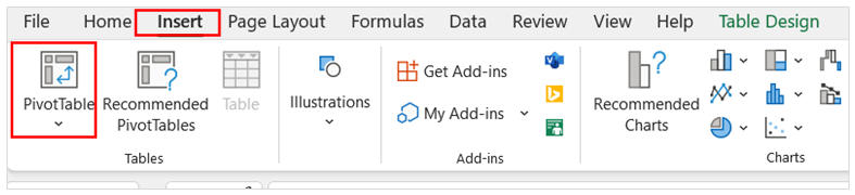
Then click on Insert menu tab and choose PivotTable
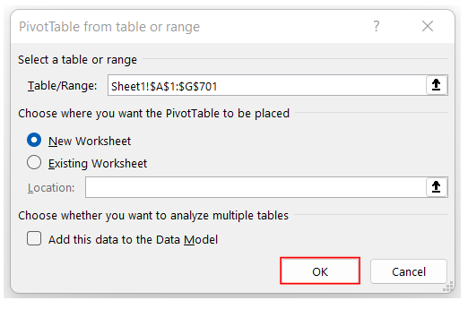
A new dialog box will appear indicating the Table/range of data and to choose an option where the pivot table will be placed.
By default, pivot table will place in a new worksheet. Click OK to create a pivot table in a new worksheet.
You can choose existing worksheet, in that case you need to select the location i.e., cell number of existing sheet (e.g., J1).
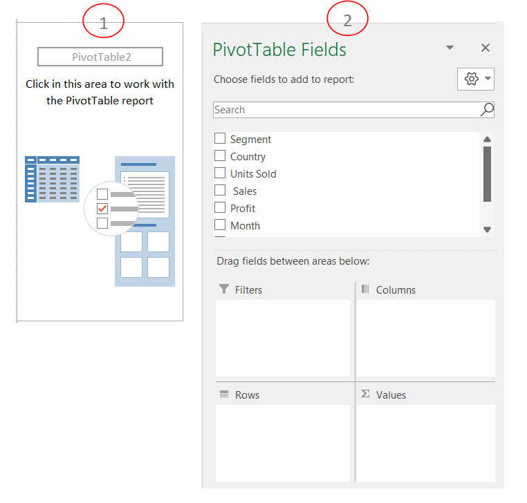
After clicking OK, two pop up menus will be appeared. First one is showing where the Pivot Table will be place and second one is showing the fields which can be included in the Pivot Table.
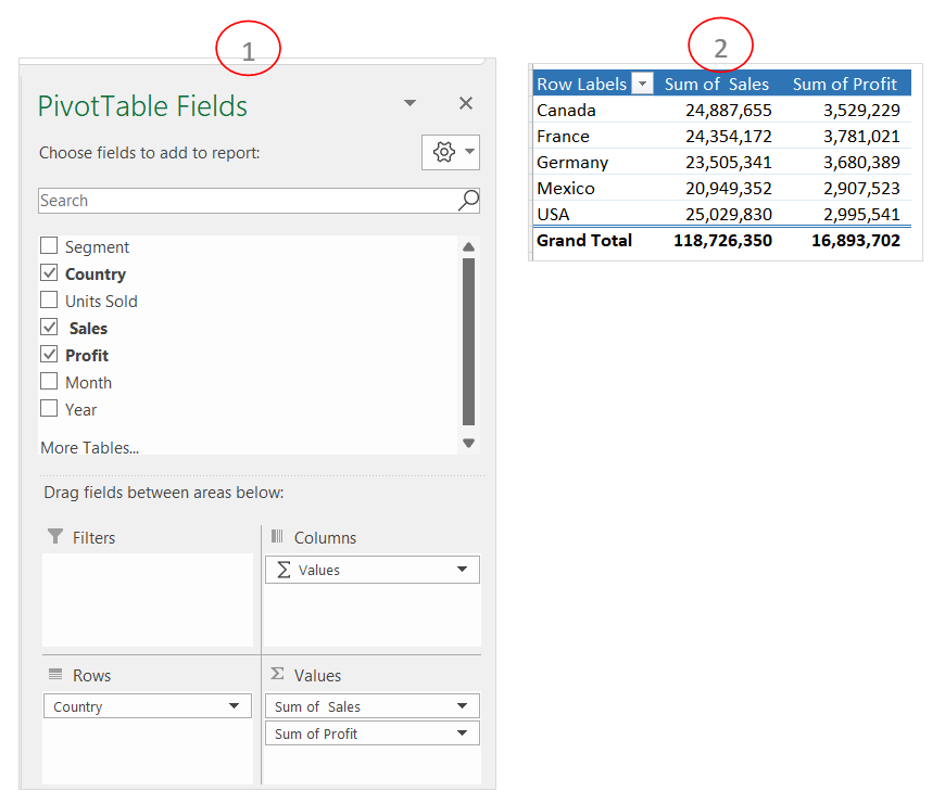
Now from second pop up drag ‘Country’ to Rows section, ‘Sales’ and ‘Profit’ to Values section. As a result, we will get the summary result of 700 columns each country’s Sales and Profit data in just 7 columns.
Add a Filter in Pivot Table
Filters in Pivot Table help you to segregate your data in more customize way. Pivot table filters work same way as Excel filters which summarize data as per selected attributes.
To create filter in Pivot Table, please see the following steps in our example:
Now drag ‘Segment’ to Filter section
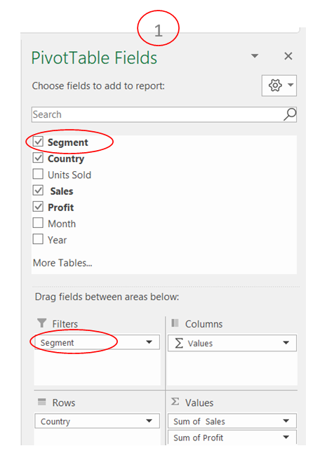
Pivot table will look like below
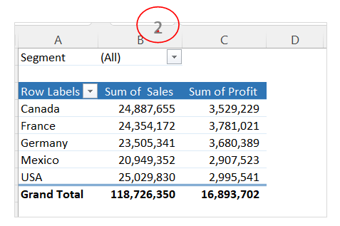
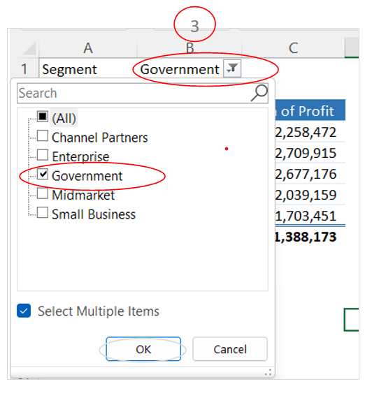
Now from Segment drop down select Government to summarize its data and click OK.
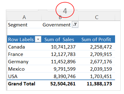
Data will be filtered by ‘Government’ segment.
You may be interested:
