A PIVOT CHART is one of the most effective ways of presenting data in Excel. Excel’s PivotChart is a built-in program tool that allows you to summarize specific rows and columns of data in a spreadsheet. We can identify negative trends and correct them quickly with the help of a PivotChart.
This Tutorial Covers:
- How to create Pivot Chart in Excel? How to construct an excel pivot chart?
- Insert Pivot Chart
- Create From Data Source
- Create From PivotTable
- How to Filter Pivot Chart Data in Excel?
- How to Change Pivot Chart Type in Excel?
- How to Refresh Pivot Charts?
- How to Move a Pivot Table in Excel? / How to Move Chart to New Sheet in Excel? / How to Move Chart to another Sheet in Excel?
- How to use a slicer with a pivot chart to filter?
- How to create Pivot Chart in Excel? How to construct an excel pivot chart?
In Excel, a pivot chart is a visual representation of data. It provides a high-level view of your raw data. It lets you evaluate data using numerous graphs and styles. It is regarded as the finest chart to use during a business presentation with large amounts of data.
| Pivot Chart | Normal Chart |
| 1. A Pivot Chart is bidirectionally linked to a PivotTable. | 1. A ‘normal’ chart is usually based on a list of data in cells. |
| 2. Filters, sorts, and data rearrangements made to Pivot Charts are also applied to their corresponding PivotTable, and conversely. | 2. Using filters, sorts, and computations on these types of charts requires modifying the source data cell formulas or inputs. |
| 3. Slicers may also be applied to PivotCharts, and a single slicer can be applied to many PivotTables/Pivot Charts if they are based on the same data. | 3. Changes to the chart have no effect on the data. |
2. Insert Pivot Chart
There are 2 ways to make a pivot chart in Excel.
- Create From Data Source
- Create From PivotTable
Steps to create a pivot chart from Data Source in excel:
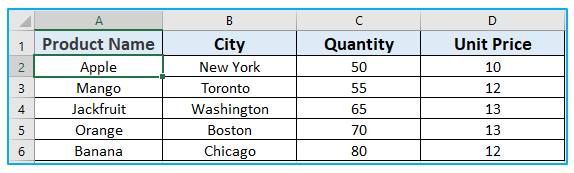
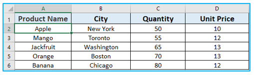
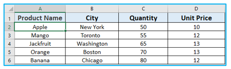
Step 1: Prepare a data table as below and select any cell in the table.
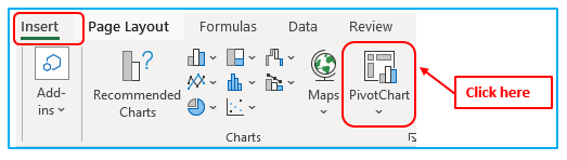
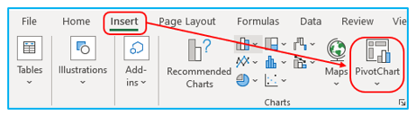
Step 2: Go to Insert. Then click on Pivot Chart.
Step 3: Either create a new sheet or specify the table range where you want the chart to be placed under Existing Worksheet.
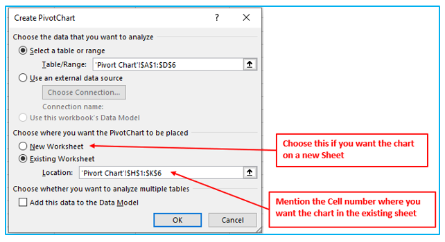
Step 4: Click OK. This will generate a blank pivot chart and pivot table. You can build a report and a chart by adding the desired fields.
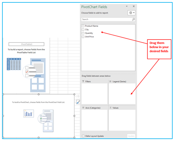
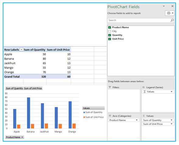
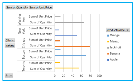
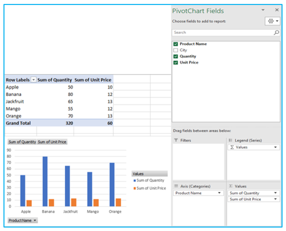
Step 5: Drag Product Name field from above mentioned picture right site box to Axis (Categories) filed. Then Drag Quantity and Unit Price to the Values filed.
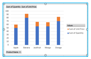
Result Outlined Below:
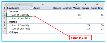
Steps to create a pivot chart from the following PivotTable in excel:
Step 1: Select any cell in PivotTable.
Step 2: Go to Insert. Then click on PivotChart.
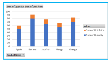
Step 3: It will provide a list of possible charts; choose the one you want (for learning select Clustered Bar).
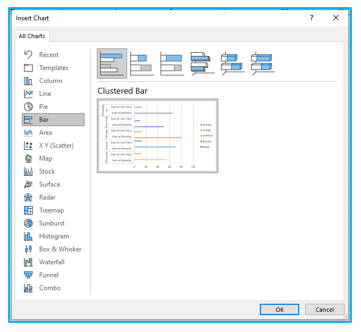
Step 4: Click OK.
Result Outlined Below:
3. How to Filter PivotChart Data in Excel? / Filter PivotChart / Filter a Pivot Chart
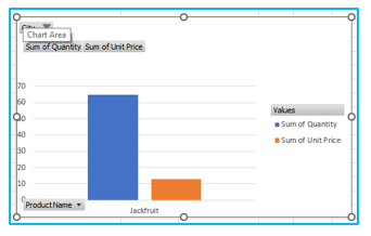
If you apply a filter to your pivot table, it will be added to your pivot chart automatically, and vice versa.
Steps to Filter Pivot Chart in Excel:
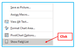
Step 1: Select any cell in pivot chart, Right-click on the chart and select “Show Field List.”
Step 2: Drag fields into the filter box of your pivot chart field list.
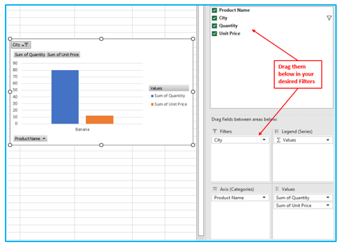
Simply drag the item’s button back to the PivotTable Fields list to remove it from the pivot chart.
Result Outlined Below:
4. How to Change Pivot Chart Type in Excel? / Change Pivot Chart Type
You can also alter the chart type by following the steps below.
Step 1: Select the pivot chart.
Step 2: Go to the Design tab, in the Type group, click on Change Chart Type.
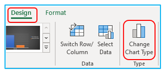
Step 3: Choose your preferred chart type.
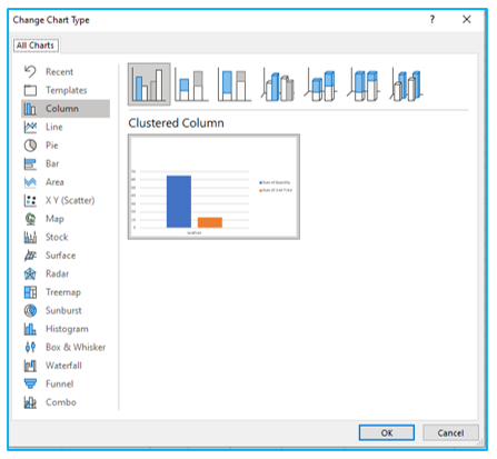
Step 4: Select a new chart type and click OK.
Result Outlined Below:
5. How to Refresh Pivot Charts? / Refresh Pivot Chart
You can update the data in your pivot chart manually or automatically, regardless of whether it comes from an external source or the same worksheet.
Option 1: Refresh a Pivot Chart Manually
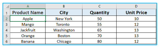
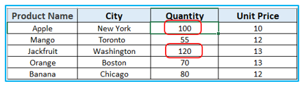
Here we have an Excel table that consists of the Product Information.
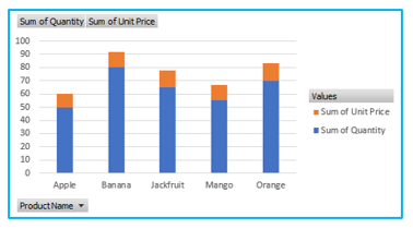
And the PivotChart looks like this:

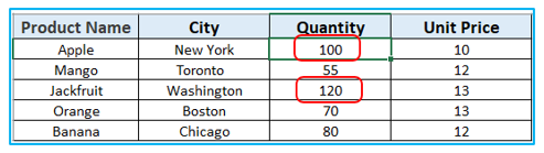
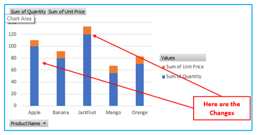
After some changes in the Table:
To Refresh the PivotChart, follow the below process:
Step 1: Select the pivotchart.

Step 2: Navigate to the PivotChart Analyze tab. In the Data area of the ribbon, select the Refresh drop-down arrow.
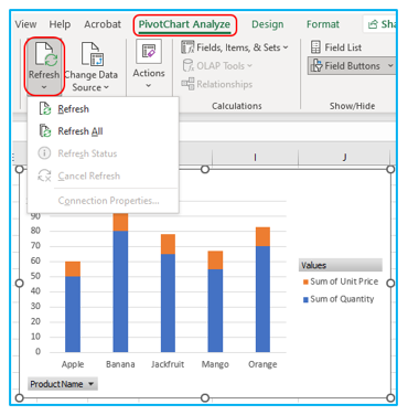
Step 3: Select “Refresh” to refresh the specified pivot chart. Choose “Refresh All” to refresh all pivot chart in your workbook.
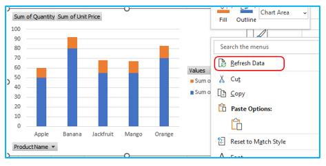
Option 2: Refresh a Pivot Chart by right click.
Here we have an Excel table that consists the Product Information.
And the PivotChart looks like this:
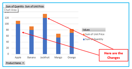
After some changes in the Table:
To Refresh a Pivot Chart by right click, follow the below process:
Step 1: Right-click the pivot chart and select “Refresh.”
Result Outlined Below:
Option 3: Refresh a Pivot Table Automatically.
Here we have an Excel table.
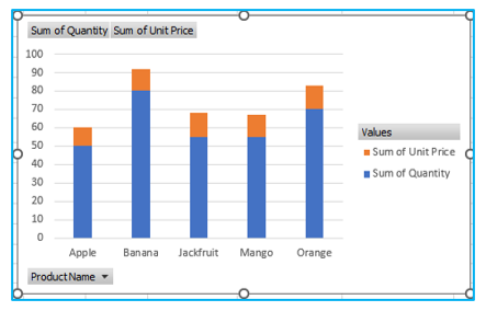
And the PivotChart looks like this:

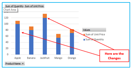
After some changes in the Excel Table:

To Refresh the PivotChart, follow the below process:
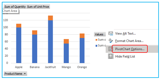
Step 1: Right-click the pivot table and select “PivotChart Option.”
Step 2: Go to the data tab and mark the box “Refresh data when opening the file.”
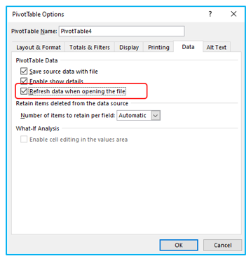
Step 3: Click Ok.
Result Outlined Below:
6. How to Move a Pivot Table in Excel? / How to Move Chart to New Sheet in Excel? / How to Move Chart to another Sheet in Excel?
Below are the steps to move a pivot chart to new sheet:
Step 1: Select the pivot chart.
Step 2: Navigate to the Design. In the Location area of the ribbon, select the Move Chart.
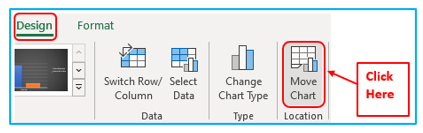
Step 3: In move chart dialog box, click on your desired option.
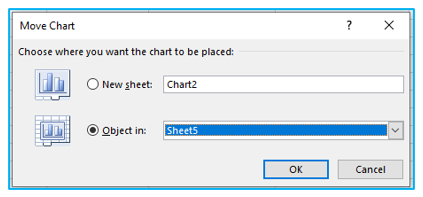
Step 4: Click Ok.
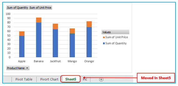
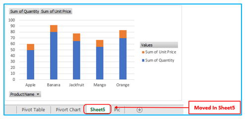
Result Outlined Below:
Option 2: Move Pivot Chart by right click.
Step 1: Right-click the pivot chart and select “Move Chart.”
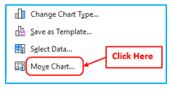
Step 2: Move chart dialog box will open. Click on your desired option.
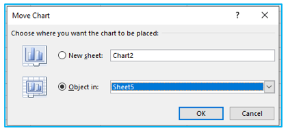
Step 3: Click Ok.
Result Outlined Below:
7. How to use a slicer with a pivot chart to filter? / Using a Slicer with a Pivot Chart to Filter.
Step 1: Select the pivot chart.
Step 2: Navigate to the PivotChart Analyze tab. In the Filter area of the ribbon, select the Insert Slicer.
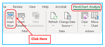
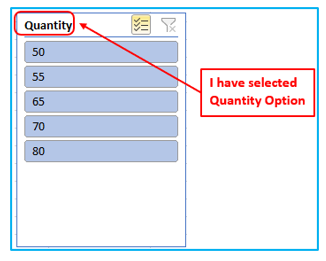
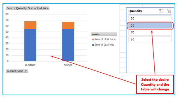
Step 3: Choose the field you want to use as a filter.
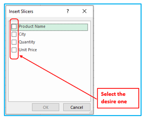
Step 4: Click Ok.
Result Outlined Below: