Create Group in Pivot Table Items to unlock advanced data analysis capabilities within your spreadsheets. This powerful feature allows you to streamline complex information into manageable segments, enhancing clarity and focus in your reports. Whether you’re looking to perform in-depth trend analysis, simplify your data presentation, or tailor your findings to specific audience needs, grouping in pivot tables provides the flexibility and precision needed for impactful data storytelling. Embrace this feature to elevate your analytical projects, ensuring that every pivot table you create delivers clear, actionable insights.
Here we will show you how you can group pivot table items. You can group the data based on Name, Date and Number. A detailed tutorial on this topic is given below.
Group Names/Products/Items
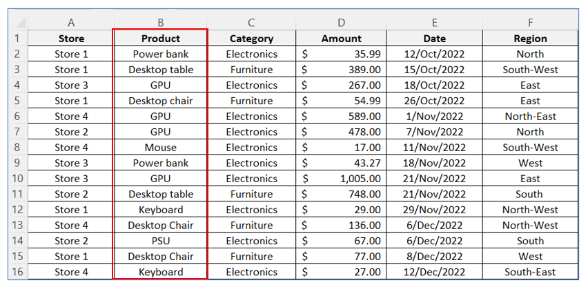
You have 7 items in the worksheet given below – GPU, Desktop table, Desktop chair, Power bank, PSU, Keyboard and mouse. Among them GPU, Power bank, PSU, Keyboard and mouse are electronic items and Desktop chair, and table are furniture items.
From the above data table, we create the following Pivot Table:
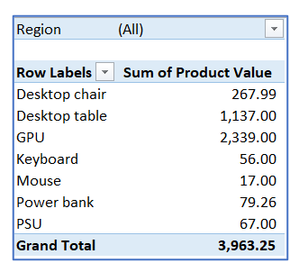
You can separate these two sort of items in two groups following the steps below.
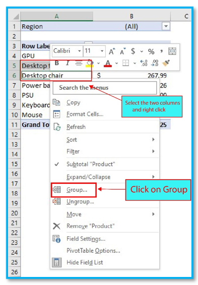
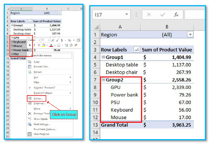
First: Press and hold Ctrl command key and select Desktop chair and Desktop table one by one and right click on your mouse. Now click on Group.
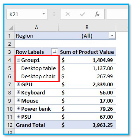
Second: Group 1 is created.
Third: Follow the same process for selection or click and drag from GPU to Mouse, then right click and select Group to create another group for the electronic items which will be Group 2.
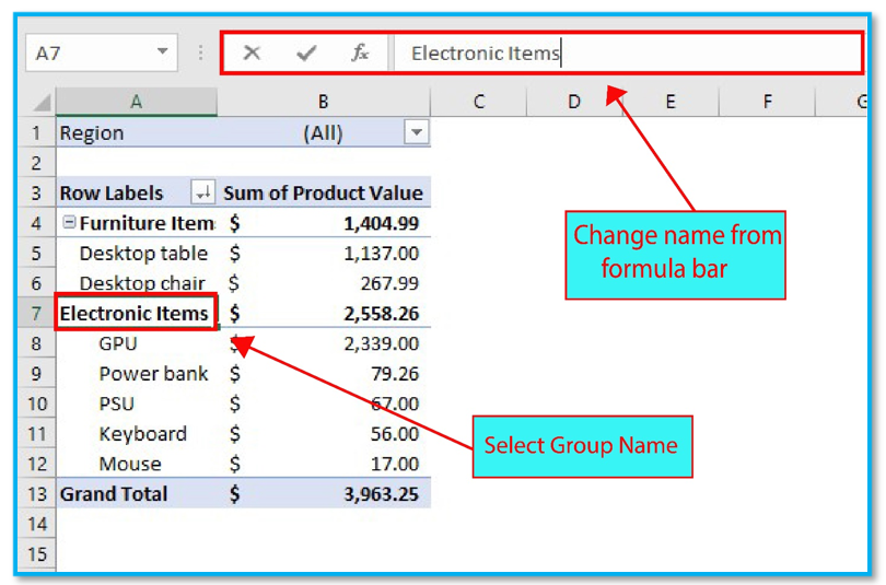
Fourth: You can also change the names of the groups. Simply click on the name of a group and then change the name from Formula bar.
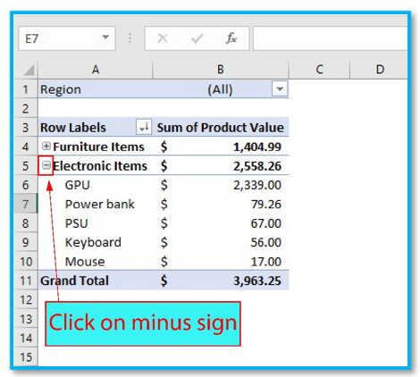
Fifth: If you want to minimize the groups just click on the minus sign.
Group Dates
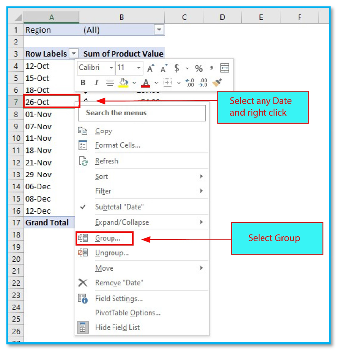
The worksheet contains many dates like 12-Oct-2022, 7-Nov-2022, 8-Dec-2022 etc. You can create groups of these dates too for your work purposes.
Step 1: Click on any cell that have dates and then right click on your mouse. Click on Group.
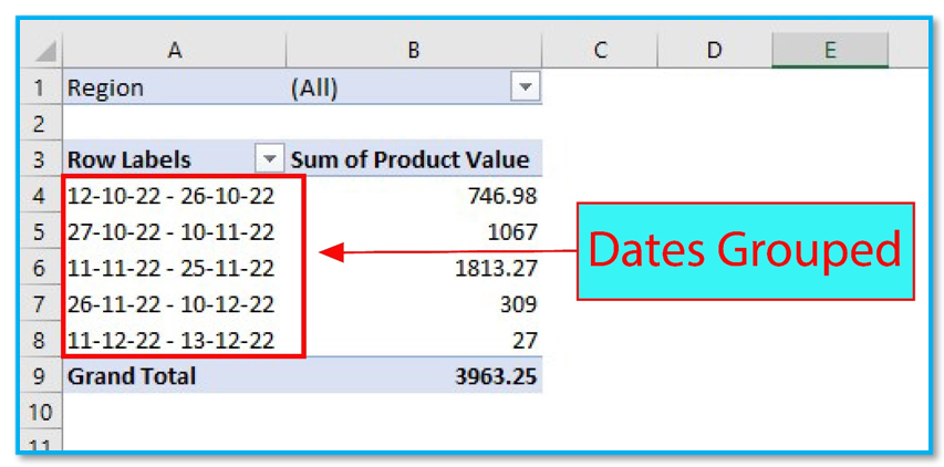
Step 2: Select Days. Type any number in the Number of days box to select the range of dates you want to create. The dates are grouped based on 15 days range in the example below.
Step 3: Here we can see 11/11/22 – 25/11/22 is the range of dates with most Sum of Product Value.
Group Numbers
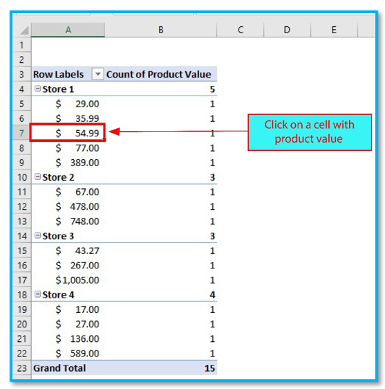
Here we will show you how you can group the data on your worksheet based on numbers. A pivot table is given below which is representing the Store no, Product value and Product amount. To create group numbers using this pivot table, follow the steps bellow.
Stage 1: Click on any cell which has Product Value in it.
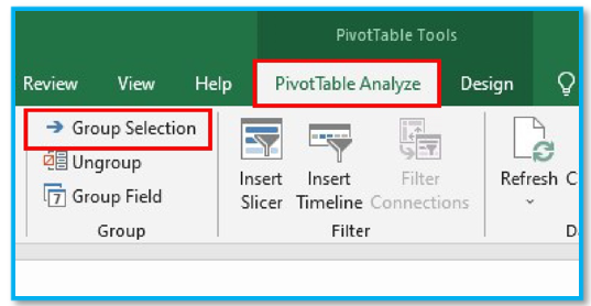
Stage 2: Now select Pivot Table Analyze and Select Group Selection.
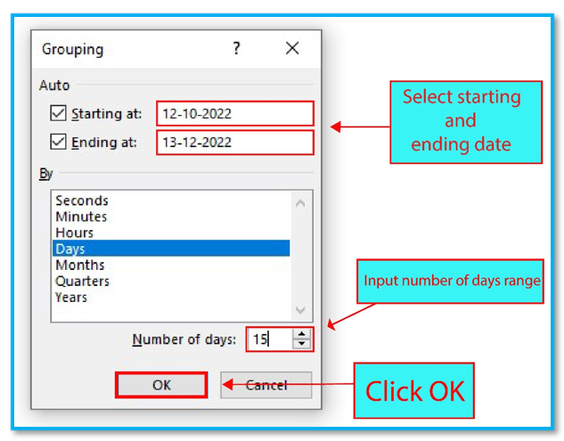
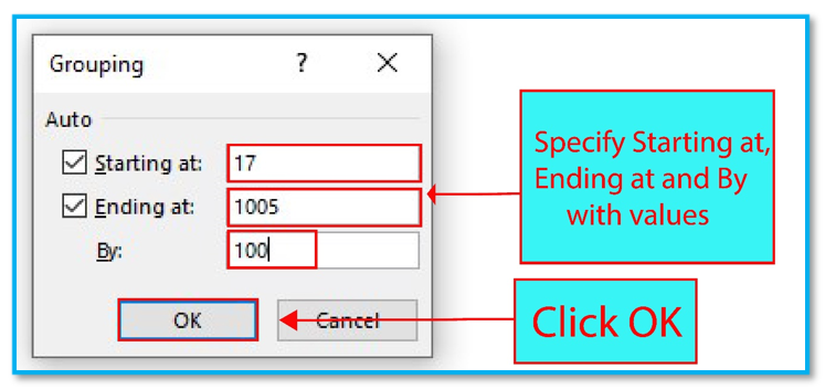
Stage 3: A Grouping dialogue box will pop-up on your screen. Specify the Starting at, Ending at and By with your desired values as shown below in the picture based on your worksheet data and click OK.
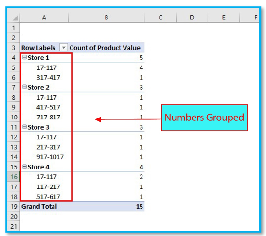
Stage 4: The data in this worksheet are Grouped based on the number range of product’s value. Here we can see Store 3 has the highest valued transaction between range $917-$1017.
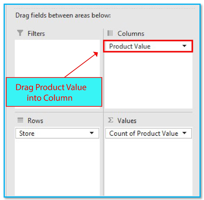
Stage 5: You can also create a matrix by dragging the grouped Product Value in column area.
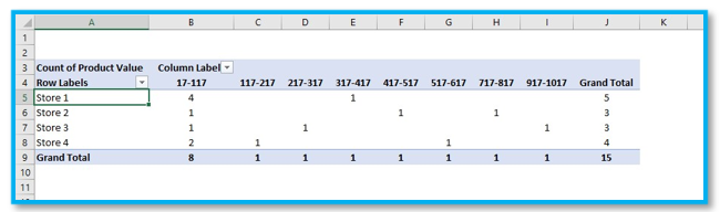
This table can be used to analyze which stores does the high value transactions and which stores need to improve on its strategy for better sales.
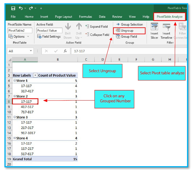
How to Ungroup Numbers in Pivot table
These number groups created above can also be Ungrouped if needed. Simply click on any grouped number and then select Pivot Table Analyze and click Ungroup.
Application of Create Group in Pivot Table Items
- Data Categorization: Use the Create Group feature in pivot table items to categorize related data into groups, making it easier to analyze subsets of data based on shared characteristics.
- Time Series Analysis: Group dates in pivot table items to analyze data over specific time periods, such as months, quarters, or years, facilitating trend analysis and forecasting.
- Range Segmentation: Create groups to segment numerical data into ranges, such as income brackets or age groups, allowing for detailed demographic analysis and targeted insights.
- Simplified Reporting: By grouping similar items, you can simplify complex data sets, making reports easier to understand and communicate to non-technical stakeholders.
- Custom Comparisons: Group different products, services, or regions to create custom comparisons and understand performance variations across different segments of your business.
- Enhanced Data Management: Use grouping to manage large data sets more effectively, reducing clutter in your pivot table and focusing attention on key areas of interest.
For ready-to-use Dashboard Templates:
