Procedure for creating dependent drop down list in Excel.
The dependent drop-down displays values in a drop-down list based on the value selected in another drop-down. This makes it simple for users to enter the data that is required. Dropdown lists are used to validate data in a unique way.
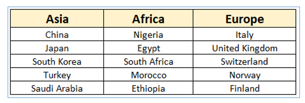
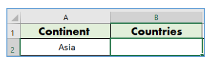
First take a sample list of Continents and some of its Counties as per below list:
Steps of creating a Dependent Drop-Down List in Excel:
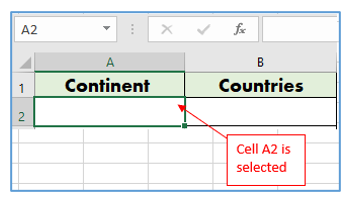
Step-1: Select the cell where you want the first (primary) drop down list to appear.
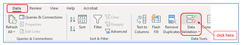
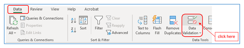
Step-2: Navigate to Data. Then tap on the Data Validation. The data validation dialog box will appear.
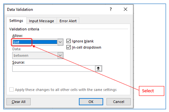
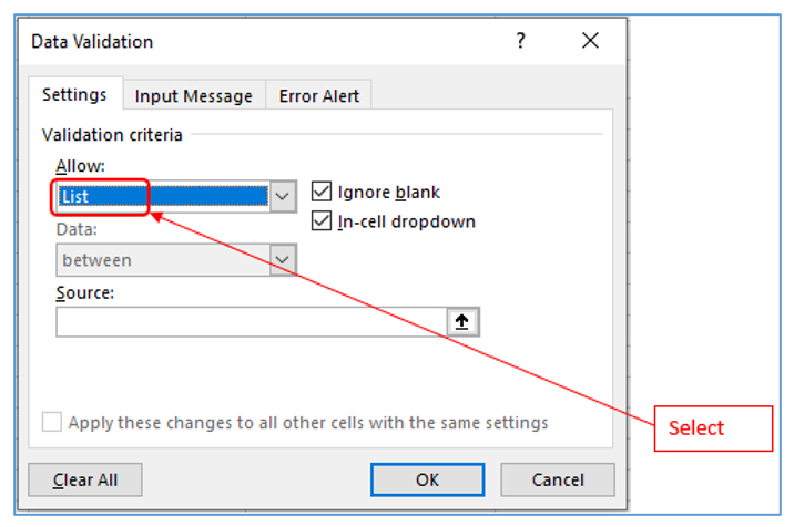
Step-3: Select List on the data validation dialog box’s settings tab.
Step-4: In the Source area, enter the range that contains the items to be displayed in the first drop down list.
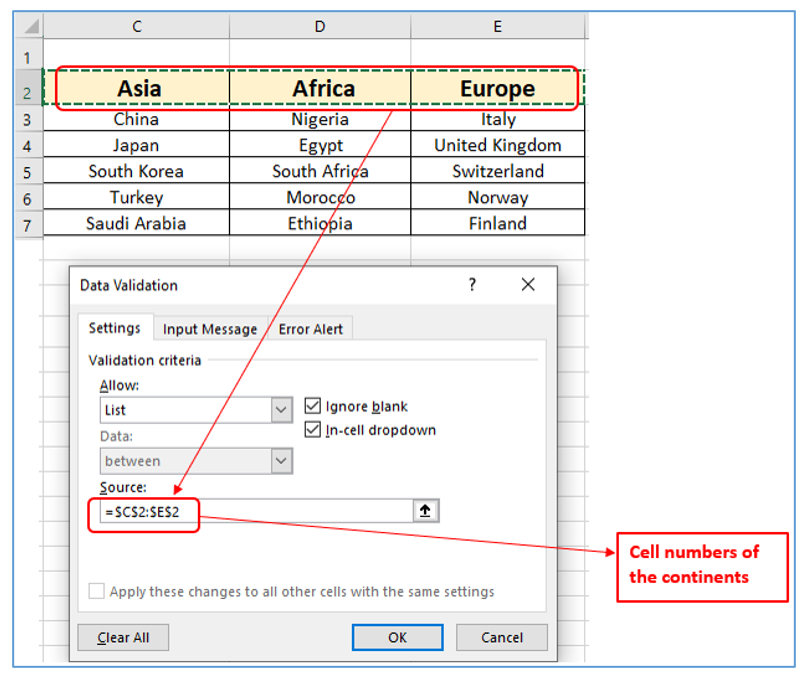
Step-5: Select OK. This will result in the creation of the Drop Down 1.
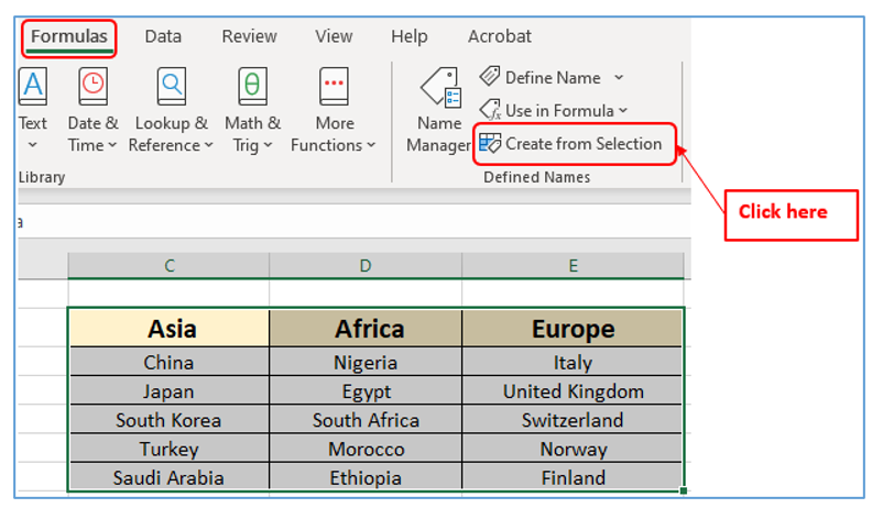
Step-6: You must build named ranges for dependent drop-down lists. Select the entire data set. Navigate to Formulas -> Defined Names -> Create from selection.
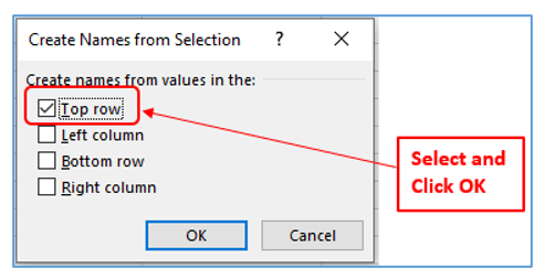
Step-7: A pop-up will appear. Select “Top Row” and then click OK.
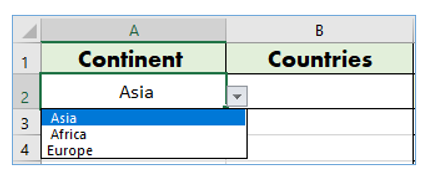
Step-8: Choose the cell where you want the Dependent/Conditional Drop-Down list to appear.
Step-9: Navigate to Data. Then tap on the Data Validation. The data validation dialog box will appear.
Step-10: Select List on the data validation dialog box’s settings tab.
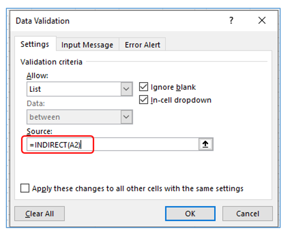
Step-11: Enter the following formula in “Source” and click OK.
=INDIRECT(A2)
(A2 is the cell that holds the main drop-down menu.)
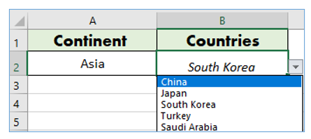
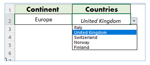
Result outlined below:
Choose Europe from the Continent list, in Countries drop you see the relevant countries.
You may be interested:
