How to create a drop down list in Excel?

Procedure for excel how to add drop down list.

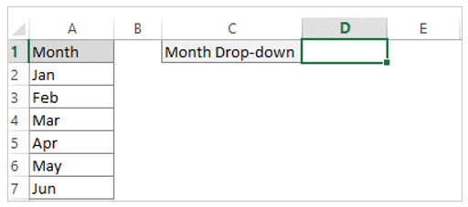
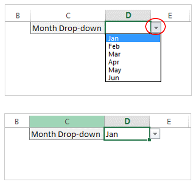
We will create the Month name drop down in cell D1. First, keep the cursor on cell D1 to show the drop-down list there.

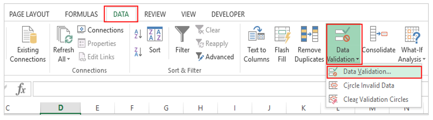
From Data Tab select Data Validation

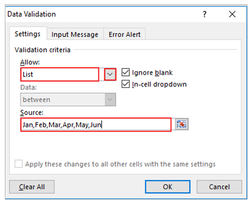
In first method we will create drop-down list through writing month name directly in the ‘Source’ box, see the below

From the Allow section select ‘List’ from the down arrow and then write month name with coma in the Source box, then click OK

You will the see the drop-down arrow in cell D1, select the month from the list.

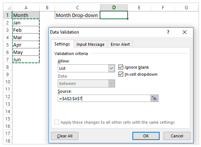
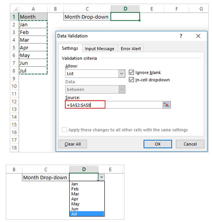
In the second method we will create drop down in Excel through referencing the source cells in the ‘Source’ box, see the below

We will create Month name dropdown list excel in cell D1. First keep cursor on cell D1 to show the drop-down list there.

From the Allow section select ‘List’ from the down arrow and then click on the Source box to refer the source data and then click OK, see below

You will the see the drop-down arrow in cell D1, select the month from the list.

Add new item or delete item from the excel drop down list

To Add new item in the drop-down list

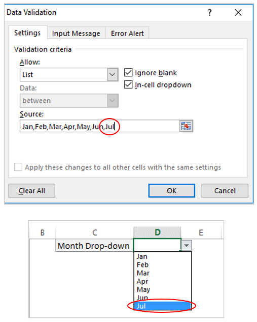
If you follow to write directly in the ‘Source’ Box then write new item after the existing items. Here we added new month Jul after the existing month names. The new month name appeared in the drop down list accordingly.

To delete item from the drop-down list

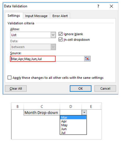
Just delete the item (here we delete Jan and Feb) from the Source box. You see the result in drop-down list in below image that Jan and Feb are no more in the drop-down list.

Add item through reference the source in the ‘Source’ Box

First add the item in the reference source, see the below that we added new month name Jul at the bottom of the table

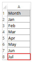
In the Source box select the source range from A1:A8 to add new month i.e., Jul in the drop-down list

If you use cell reference as source to create drop-down, to delete the item you just remove the cell/cells from the reference source and drop-down will updated automatically.

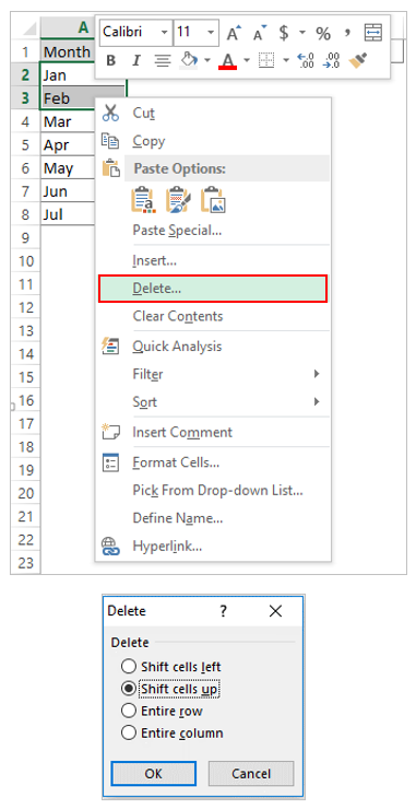
Say, we want to remove Jan and Feb from the drop-down list

Select the Jan and Feb cells, then right click and select Delete. From the Delete pop up select ‘Shift cells up’. Jan and Feb month deleted from the table.

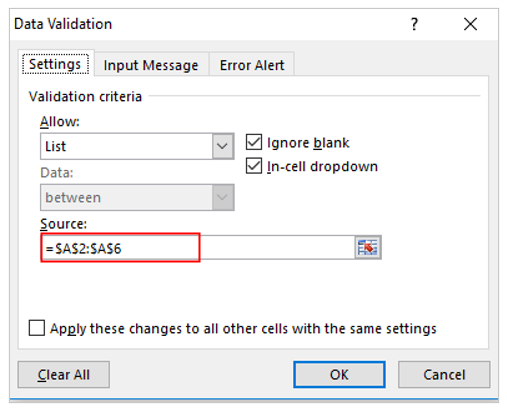
The drop down is update automatically

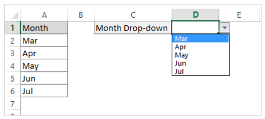
See the source reference in the Source Box, source reference adjusted to range A2:A6 before which was A2:A8

Dynamic drop down – how to create drop down menu in Excel?

Select the cell (here D1) where you want to create the drop-down

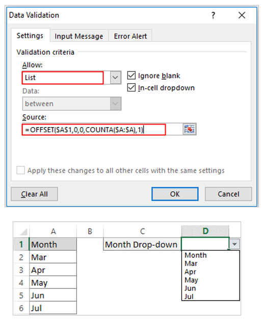
In Data Validation window write following OFFSET formula in Source

=OFFSET ($A$1,0,0, COUNTA ($A: $A),1)

And click OK.

How OFFSET function works in Excel?

Syntax of OFFSET function: OFFSET (reference, rows, cols, [height], [width])

Total 5 arguments are used in OFFSET function. In our example arguments are:

Reference: A1 is the reference cell

Rows: number of rows up or down. We move 0 rows up or down

Cols: number of calls to left or right. We are using single col so 0 col

Height: we use COUNTA function in col A:A to count the values in col A that are not empty.  When you add one item in the list COUNT(A:A) considers it accordingly.

Width: here width is 1

Now if you add two more months in our monthly list say add Aug and Sep then drop-down will be adjusted dynamically.

 

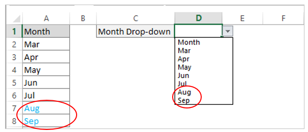
Aug and Sep are added in the month list which are reflected in the drop-down list.

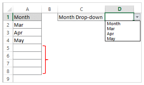
Now we delete Jun, Jul, Aug, and Sep from the month table, in the right-side drop-down list updated accordingly

How to use Excel Table to create dynamic drop down list?

To create Excel Table, click any cell of Month list and press CTRL+T then Create Table pop up appears and click OK

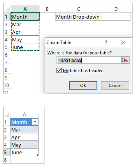
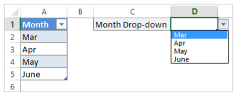
Here our Excel Table name is ‘Table1’ and column name is ‘Month’

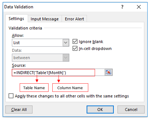
Now use the Excel Table reference in Data Validation Source to make the dynamic drop-down. We will use INDIRECT function to create the reference.

Drop-down list looks like below

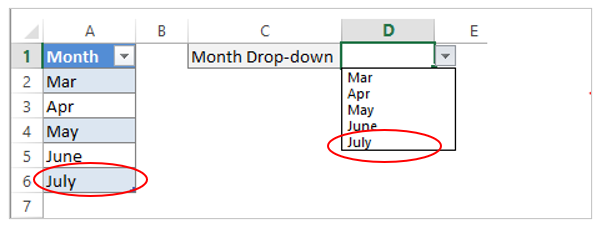
Now if you add July in the table, the drop-down will be adjusted dynamically.

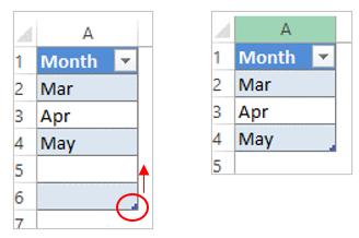
If you delete any month form the table, you need to adjust the excel table accordingly.

Drag the bottom right corner icon to last month’s cell.

You may be interested:

1. Financial Dashboards
2. Sales Dashboards
3. HR Dashboards