Copy Conditional Formatting to Another Cell in Excel is a game-changing feature that brings dynamic interactivity to your spreadsheets. By setting up rules based on the values of other cells, you can create visually intuitive dashboards, highlight critical data points, and automate the visual representation of changes and trends. This powerful tool not only enhances your data’s readability but also aids in faster decision-making and error detection. Harness the capability of conditional formatting linked to other cells to transform your data analysis, making your Excel projects more efficient and insightful than ever before.
This Tutorial Covers:
- How to copy Conditional Formatting Using Paste Special in Excel
- How to copy Conditional Formatting Using Format Painter in Excel
- Issues when Copying Conditional Formatting
1. How to copy Conditional Formatting Using Paste Special in Excel?
The conditional formatting can be copied and pasted from one cell to another just like you can copy and paste cells within the same sheet or even between sheets or workbooks.
The cell cannot be copied and pasted, as you may have noticed. Make sure to only copy and paste the conditional formatting rules into a cell after copying it (and not everything else, such as the value or the formula).
You must utilize Paste Special and ensure that you only copy and paste the conditional formatting.
Assume you have a dataset like the one below, where I’ve used conditional formatting to column B (the English score) to highlight any cells with a value lower than 60.

What if I wanted to use the same conditional formatting rule for the second column (which is for the Math score) such that all the cells below 60 were highlighted?
This is simple to accomplish!
The procedures to copy conditional formatting from one cell to another are described below:
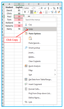
Step 1: Choose cell B4 and then right-click it and choose “Copy” (or press the shortcut “Control + C”)
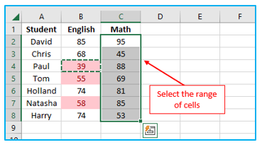
Step 2: Choose the complete range where you wish to duplicate the conditional formatting (C2:C8 in this example)
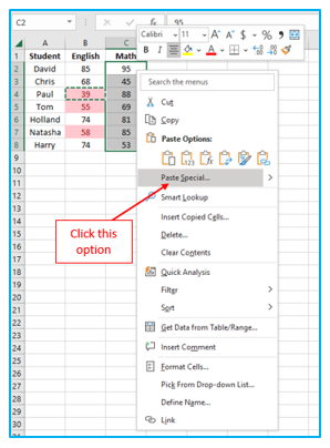
Step 3: Anywhere in the selection, click with the right mouse button. Select “Paste Special” from the menu. The “Paste Special” dialog box will then be displayed.
Step 4: Select “Formats” from the “Paste Special” dialog box and then select “OK”
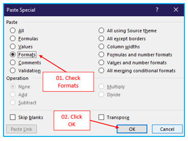
By following the steps above, the conditional formatting from column B would be copied and applied to the chosen cells in column C.
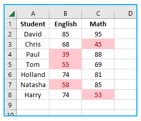
One thing to keep in mind is that Paste Special will copy all formatting when you use it to copy conditional formatting. Therefore, any borders or bold text that may be present in the cells would likewise be copied.
Note:
When copying and pasting conditional formatting to cells in another sheet or even another workbook, the same procedures as before would apply.
2. How to copy Conditional Formatting Using Format Painter in Excel?
Using the tool known as “Format Painter,” you can copy the format from a cell (or range of cells) and then paste it.
You may also use format painter to copy and then paste conditional formatting because it is a component of formatting as well.
Imagine you had a dataset like the one below, where I’ve applied conditional formatting to the English score column to highlight any cells with a value lower than 60.
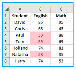
Following are the instructions for using Format Painter to copy conditional formatting in excel from one cell to another:
Step 1: Choose the cell (or group of cells) from which you want to replicate the conditional formatting.

Step 2: Click the “Home” tab and simply select the “Format Painter” icon under the “Clipboard” group.
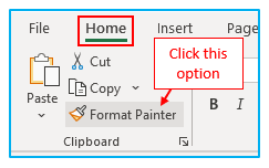
The cursor transforms into a painter icon, as shown below.
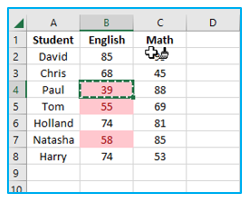
Step 3: Choose every cell where you want to use the copied conditional formatting. The result looks like below.
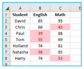
The format painter can be used on the same sheet, another sheet in the same workbook, or even on a different workbook once it has been active.
Format painter also replicates all the formatting, just like paste special did (including the conditional formatting).
Pro tip: Click on the Format painter icon twice if you want to copy the conditional formatting and paste it on numerous cells or ranges (that you can’t pick all at once). By doing so, you can continue using the format painter and repeat the formatting process (unless you hit the Escape key).
3. Issues when Copying Conditional Formatting
Conditional formatting can typically be copied and pasted from one cell to another without any issues.
However, if you chose specific cells to format using a custom formula, you might run into problems.
The formatting is applied when the formula returns TRUE for a cell and is not applied when the formula returns FALSE when using this option, which enables you to construct your own formula.
If you have used absolute or mixed references in a formula for conditional formatting, it might not copy correctly.
For instance, in the example below, I have highlighted all cells in column B with values lower than 60 using the formula =$B2=60.
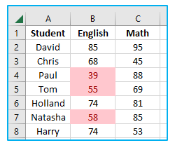
However, it still refers to the B column when I duplicate this conditional formatting to column C, and the outcome is incorrect (as shown below).
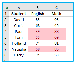
So, it’s recommended to examine the formula and update the references if you copy conditional formatting from one cell to another and don’t get the desired result.
For instance, if I modify the formula in this instance to =B2=60, everything should be good.
In case you’re wondering where the formula is placed, select “Conditional Formatting” from the “Home” tab. Select “New Rule” from the list of possibilities that appears. Select the “Use a formula to select which cells to format” option in the “New Formatting Rule” dialog box.
You will see the field where you can enter the formula for the chosen range when you do this. The cell will be formatted if this formula returns TRUE for it; else, it will not.
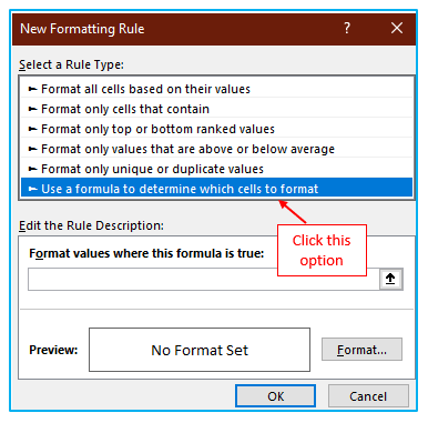
Therefore, using Paste Special and Format Painter, you can replicate conditional formatting from one cell to another in Excel.
Check the custom formula that was used in it if you notice any problems with it.
Application of Copy Conditional Formatting to Another Cell in Excel
- Visual Data Tracking: Apply conditional formatting to a cell based on the value of another cell to visually track changes or statuses, such as highlighting due dates that are approaching based on today’s date.
- Performance Indicators: Use conditional formatting to change the color of a performance indicator cell based on the target achievement rate entered in another cell, enabling quick assessment of goal attainment.
- Budget Monitoring: Highlight budget cells in red if the expense in a corresponding cell exceeds the set budget limit, allowing for immediate identification of financial overruns.
- Inventory Level Alerts: Set up conditional formatting to alert when inventory levels in one cell fall below a minimum threshold defined in another cell, facilitating timely restocking.
- Task Completion Status: Change the color of task status cells based on completion percentage entered in another cell, providing a clear visual of project progress.
- Temperature Ranges: Apply conditional formatting to display temperature data in different colors based on predefined temperature ranges in separate cells, aiding in climate or environmental analysis.
You may be interested:
