Convert Month Name to Number in Excel concludes your quest for streamlined data processing and date management. This transformational technique not only enhances the consistency of your datasets but also unlocks advanced sorting, searching, and analytical functionalities. Embrace the power of converting month names to numbers in Excel to elevate your data organization to new heights of efficiency. Let this skill pave the way for more accurate time-based analyses and intuitive data interactions, ensuring your spreadsheets reflect precision, clarity, and top-notch professionalism.
It’s feasible that we’ll need to convert a month to a number while using Microsoft Excel for a variety of reasons. We frequently have to convert to numbers for computation purposes.
There are 3 ways to convert Month Name to Number. They are-
1. Use MONTH Function to convert Month name to Number
It’s relatively normal to convert a date to a month name, however there may occasionally be a requirement to convert a month name to the appropriate month number.
For example, you might want to transform the month name January, June, or July in a cell to the corresponding month numbers (which would be 1 for January, 6 for June or 7 for July).
It’s possible that you need to do this to just satisfy a formatting requirement, or perhaps you need to use it to make some computations.
Procedure of convert Month Name to Number using MONTH Function:
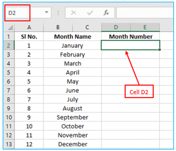
Step 1: The first step is to select a cell. I’ve chosen this cell (D2), outlined in Red below.
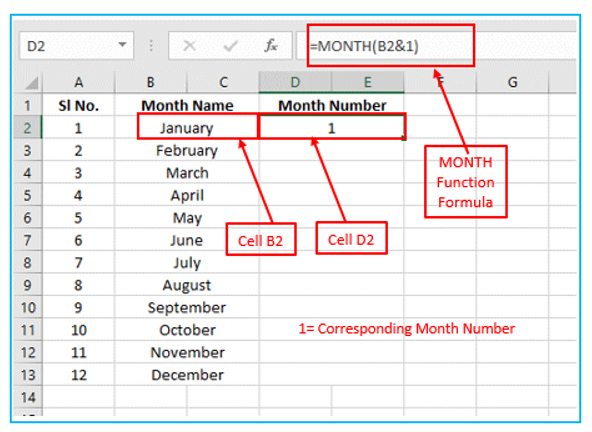
Step 2: Apply the formula for MONTH Function. The formula for the MONTH Function is outlined in Red below.
Here, The MONTH function returns a number from a given date that ranges from 1 to 12.
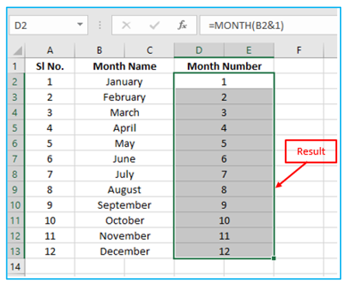
Step 3: After applying, to fill all the cells, pull the “Fill Handle” further. The result is outlined in Red below.
Using MONTH Function, you can also find Month by number, Month with number, what number month is July, what month number is June, what number month is June.
2. Combine MONTH and DATEVALUE Functions
Procedure of converting Month Name to Number by combining MONTH Function and DATEVALUE Function:
Step 1: The first step is to select a cell. I’ve chosen this cell (D2), outlined in Red below.
Step 2: Combining the formula for MONTH Function and DATEVALUE Function. The combining formulas is outlined in Red below.
Here, within the given string, the DATEVALUE function produces a date-time code.
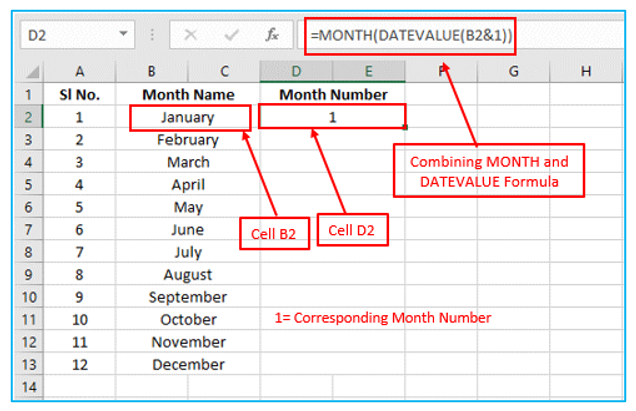
Step 3: After combining, to fill all the cells, pull the “Fill Handle” further. The result is outlined in Red below.

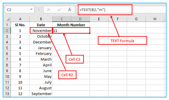
3. Apply Excel TEXT Function to Covert Month Name to Number in Excel
It’s possible to come across dates in different cells while using Microsoft Excel. You must now be considering how to transform them. Not to worry. To obtain your answer, follow the steps below.
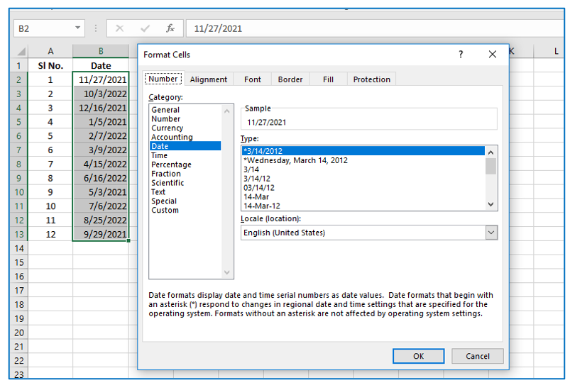
Step 1: First of all, choose all dates and press Ctrl+1 on the Keyboard. A new window is named “Format Cells”, outlined in Blue below.
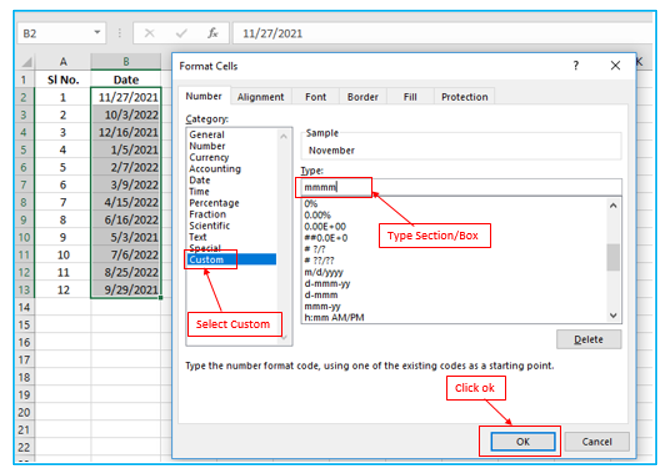
 Step 2: Select custom and write “mmmm” in the “Type” section/box and then click ok to continue, outlined in Red below.
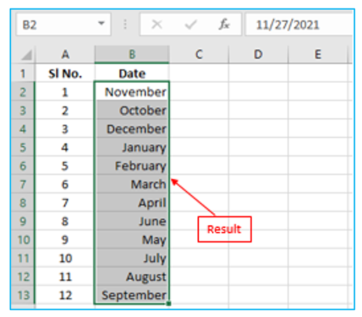
The result is outlined in Red below.
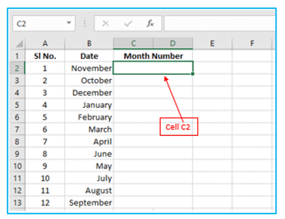
Step 3: Select the cell C2, outlined in Red below.
Step 4: Apply the formula for TEXT Function. The formula for the TEXT Function is outlined in Red below.
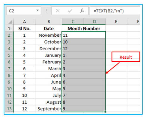
Step 5: After applying formula, to fill all the cells, pull the “Fill Handle” further. The result is outlined in Red below.
Application of Convert Month Name to Number in Excel
- Simplifying Date Sorting:
- Convert month names to numbers to enable straightforward chronological sorting of data, ensuring that datasets are organized in a logical, time-based sequence.
- Facilitating Data Analysis and Reporting:
- Use month numbers in formulas and pivot tables for more efficient and accurate monthly data analysis, comparison, and aggregation, enhancing the clarity and effectiveness of reports.
- Improving Data Integration:
- Standardize date formats by converting month names to numbers, ensuring consistency when integrating or comparing datasets from different sources or systems.
- Enabling Time-Based Calculations:
- Perform time-based calculations, such as determining durations or intervals, more effectively by using month numbers, which are easier for Excel to interpret and calculate.
- Streamlining Chart Creation:
- Create more coherent and interpretable charts by using numerical month representations, allowing for better trend visualization and time series analysis.
- Optimizing Data Storage and Performance:
- Minimize data storage space and improve performance by replacing text-based month names with numerical representations, which are more compact and efficient for Excel to process.
Converting month names to numbers in Excel enhances data manageability and opens up a wide range of analytical possibilities, making it a valuable technique for anyone looking to optimize their use of Excel for time-based data analysis.
For ready-to-use Dashboard Templates:
