Compare Text in Excel is a fundamental task for data validation, error checking, and analysis. By utilizing Excel’s built-in functions and formulas, users can efficiently compare text strings to identify discrepancies, duplicates, or patterns. This process is essential for maintaining data accuracy, ensuring consistency across datasets, and facilitating decision-making. Whether used for quality assurance, data cleansing, or record reconciliation, comparing text in Excel empowers users to detect and resolve inconsistencies effectively. Embracing this functionality enhances data integrity and reliability, streamlines workflows, and improves overall efficiency in data management tasks. With the ability to quickly and accurately compare text in Excel, users can confidently navigate complex datasets, mitigate errors, and derive actionable insights to drive organizational success.
This Tutorial Covers:
- Compare Text in Excel (Exact Cell against Cell Comparison)
- Using the Equal to Operator
- Using the EXACT function
- Using the EXACT with IF statement
- Using VLOOKUP, compare text and locate missing text
- Compare Text and Check If Partial Text Matches
1. Compare Text in Excel (Exact Cell against Cell Comparison):
Suppose you have a dataset that contains student information, including their names and corresponding student IDs. You want to compare the names in one column with the names in another column and determine if they are an exact match.
Let’s examine three quick methods for completing this.
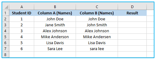
-
Using the Equal to Operator:
If two cells have exactly the same text in them, the equal operator will compare the contents of the two cells and return TRUE; otherwise, it will return FALSE.
The steps to compare text in Excel using “Equal to” operator are described below:
Step 1: Apply the below formula that will compare the text in two cells in the same row in cell D2 and you can either copy and paste the formula or drag the formula’s fill handle to the remaining cells.
=B2=C2
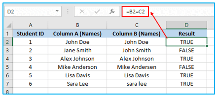
The formula above gives a TRUE if the names are an exact match (i.e., they are the same exactly) and a FALSE if they are not.
You can see from the aforementioned example that the formula in cells D2 and D4 returns FALSE, proving that the names in rows #2 and #4 are different.
You can apply filters to the headers and then limit the results to just the cells in column D with the value FALSE if you only want to view the rows where the names are different.
Note: The cell contents must perfectly match for the formula to produce a TRUE. Even if it appears as though the cells have the same name when there is an additional space in one of them, the formula will return a FALSE.
The case of the text in the cell is not considered when using the equal to operator.
The formula will yield a TRUE if, for instance, you have “Sara Lee” in B7 and “sara lee” in another cell C7 and compared the two.
Use the EXACT function technique described in the following section if you want the comparison to be case-sensitive.
-
Using the EXACT function:
Utilizing Excel’s EXACT function is yet another simple method for comparing two texts in Excel.
As its name implies, it would return TRUE if the contents of the two cells under comparison were exactly the same and FALSE if they weren’t.
Assume you use the same dataset as in the previous example.
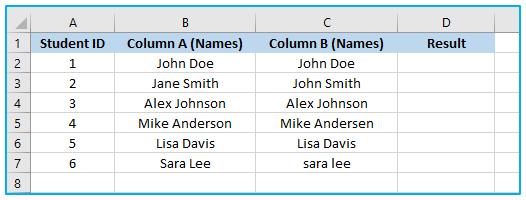
The steps to compare text in Excel using EXACT function are described below:
Step 1: Apply the below formula that will compare the text in two cells in the same row in cell D2 and you can either copy and paste the formula or drag the formula’s fill handle to the remaining cells.
=EXACT(B2,C2)
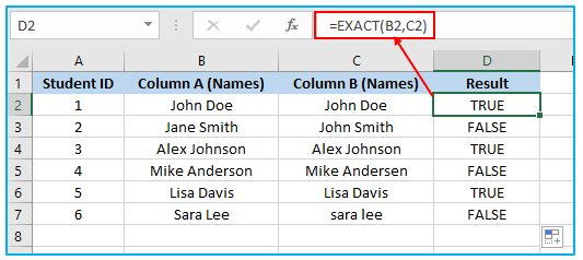
Being cognizant of the fact that the EXACT function is case sensitive, the formula would return a FALSE even if the names were precisely the same but in different cases (lower or upper, or proper).
-
Using the EXACT with IF statement:
Using the EXACT function within an IF statement to compare text in Excel and determine if two cells contain an exact match:
In this example, let’s assume you have the following dataset as in the previous example:
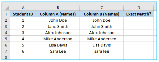
To fill in the “Exact Match?” column with “Yes” or “No” based on whether the names in Column A and Column B an exact match are, follow these steps:
Step 1: Apply the below formula that will compare the text in two cells in the same row in cell D2 and you can either copy and paste the formula or drag the formula’s fill handle to the remaining cells.
=IF(EXACT(B2, C2), “Yes”, “No”)
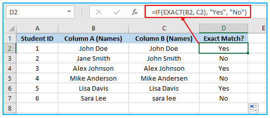
The “Exact Match?” column now uses the “Yes” and “No” labels to indicate whether or not the names in Column B and Column C are an exact match.
The EXACT function is used to compare the values in cells B2 and C2 in the formula =IF(EXACT(B2, C2), “Yes”, “No”). It returns “Yes” if the values exactly match; else, it returns “No”.
2. Using VLOOKUP, compare text and locate missing text:
When you have a list in two columns and want to identify the things or names that are present in one column but not in the other, that is another circumstance in real life where you could need to compare text.
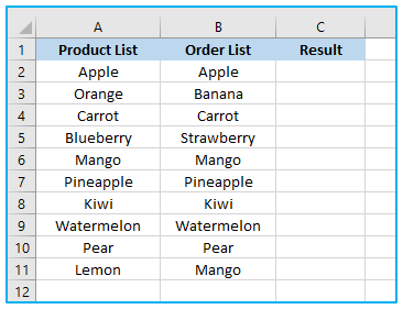
The steps to compare texts and find missing text using VLOOKUP are described below:
Step 1: Apply the below formula in cell C2 and you can either copy and paste the formula or drag the formula’s fill handle to the remaining cells.
=IF(ISERROR(VLOOKUP(B2, A:A, 1, FALSE)), “Missing”, “Present”)
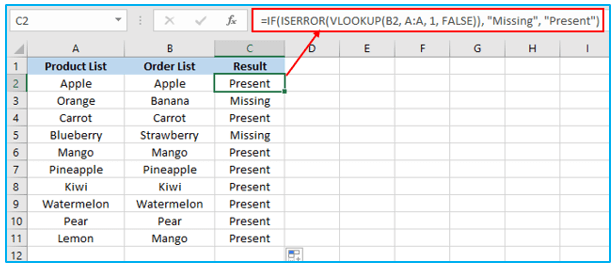
In this example, various products in the “Product List” column and corresponding orders in the “Order List” column. The “Result” column indicates whether the product is missing or not.
This formula is used in the “Result” column. It searches for each product in the “Order List” column (cell B2) within the “Product List” column (range A:A). If a match is not found, it returns an error value, which triggers the ISERROR function. The IF function then checks for the error value and returns “Missing” if there is an error or “Present” if there is no error.
In the given example, the products “Banana” and “Strawberry” in the “Order List” column are missing from the “Product List” column, as indicated by the “Missing” result. All other products have a match, so return “Present” in the “Result” column.
3. Compare Text and Check If Partial Text Matches:
Think of a dataset with a column A list of products and a column B list of keywords. We want to know if any of the keywords in Column B are included in the product names in Column A as partial matches.
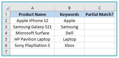
Depending on whether any of the keywords in Column B are discovered as partial matches inside the related product names in Column A, you may either put “Yes” or “No” in the “Partial Match?” column by doing the following the steps:
Step 1: Apply the below formula that will compare the text in two cells in the same row in cell D2 and you can either copy and paste the formula or drag the formula’s fill handle to the remaining cells.
=IF(ISNUMBER(FIND(B2, A2)), “Yes”, “No”)
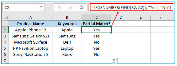
Now, the “Partial Match?” column indicates whether any of the keywords in Column B are found as partial matches within the corresponding product names in Column A.
Application of Compare Text in Excel
- Data Validation: Comparing text in Excel facilitates data validation processes to ensure accuracy and consistency in data entry.
- Error Checking: It helps identify discrepancies or inconsistencies between text strings, aiding in error detection and correction.
- Duplicate Detection: Users can compare text in Excel to identify duplicate entries or records, streamlining data cleansing tasks.
- Pattern Recognition: Comparing text enables users to identify common patterns or trends within datasets for further analysis.
- Record Reconciliation: It assists in reconciling records or datasets by highlighting differences between corresponding text values.
- Quality Assurance: Comparing text in Excel serves as a quality assurance measure, ensuring data integrity and reliability in spreadsheets.
You may be interested:
