Apply Formula to Entire Column effortlessly signifies the epitome of productivity and precision in your Excel tasks. This powerful feature streamlines your data processing, ensuring consistency and accuracy across your entire dataset. By mastering how to apply formulas to entire columns, you transform your workflow, enabling swift calculations and analysis over extensive data ranges. Let this capability be your strategic advantage in Excel, turning complex data into actionable insights with just a few clicks, and propelling your spreadsheets towards unparalleled efficiency and effectiveness.
The good news is that applying your formula quickly and easily to a complete column of cells only requires a few clicks.
This Excel apply formula to entire column tutorial shows how to use a formula across an entire column.
This Tutorial Covers:
- By Double-Clicking on the AutoFill Handle
- By Dragging the AutoFill Handle
- Using the Fill Down Option, which is located in the ribbon
- Making the Fill Down available in the Quick Access Toolbar
- Using the Keyboard Shortcut
- Using Array Formula
- By Copy-Pasting the Cell
1. By Double-Clicking on the AutoFill Handle
The use of this straightforward mouse double-click technique is one of the simplest methods to Apply Formula to Entire Column in Excel.
Consider the following dataset, where you want to enter the profit for each product in Column E.
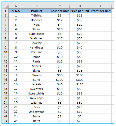
The steps for using this formula on all of columns E are listed below:
Step 1: Enter the following formula in cell E2:
=D2-C2
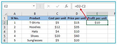
Step 2: After you select the cell, a tiny green square will appear in the bottom-right corner of the cell selection. Put the cursor over the tiny green square. The cursor transforms to a plus sign, as you will see (this is called the autofill handle)
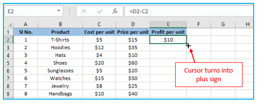
Step 3: Press the left mouse button twice. After that, the result looks like below:
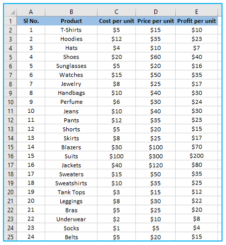
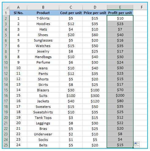
The aforementioned actions would instantly fill the column up to the cell containing the data from the adjacent column. The formula would be applied up to cell E25 in our case.
The neighboring column must be empty of any data and contain no blank cells in order for this to function. This auto-fill double click would only apply the formula to the blank cell if there was a blank cell in the column.
It’s the same as manually pasting the formula when applying the autofill handle to the full column. This implies that the formula’s cell reference would adjust appropriately.
For instance, if the reference is absolute, it would not change as the formula is applied to the column; however, if the reference is relative, it would change as the formula is applied to the cells below.
2. By Dragging the AutoFill Handle
The above double-click procedure had the drawback of stopping as soon as it reached a blank cell in one of the adjacent columns.
You can also manually drag the fill handle to apply formula to entire Column if you only have a small amount of data.
The steps to apply Excel formula in column E are described below:
Step 1: Enter the following formula in cell E2:
=D2-C2
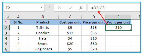
Step 2: When a cell is chosen, a tiny green square will appear in the bottom-right corner of the selected cells. Put the cursor over the tiny green square. The cursor transforms to a plus sign, as you will see (this is called the autofill handle)
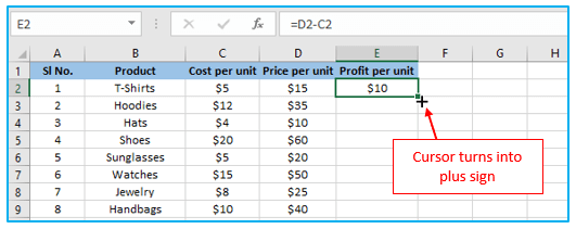
Step 3: Holding down the left mouse button, drag it to the cell where you need to apply the formula. When finished, leave the mouse button.
3. Using the Fill Down Option, which is located in the ribbon
Using the fill down option in the ribbon is another way to apply a formula to the entire column.
You must first choose the cells in the column where you want the formula to appear for this technique to function.
How to apply formula in entire column E using fill down technique is shown below:
Step 1: Enter the following formula in cell E2:
=D2-C2
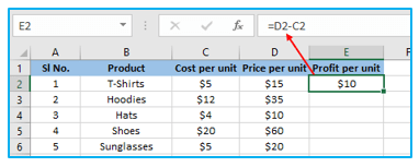
Step 2: To implement the formula, select each and every cell (including cell E2).

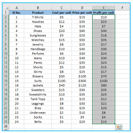
Step 3: On the “Home” tab, click. Select the “Fill” icon under the “Editing” category. On “Down”, click.

The formula from cell E2 would be copied in the above steps and entered into each of the chosen cells.
- Making the Fill Down available in the Quick Access Toolbar
If you frequently need to use the fill-down option, you can put it on the Quick Access Toolbar so that you can access it with just one click and that it is always visible on the screen.
Procedure of making the Fill Down available in QAT is shown below:
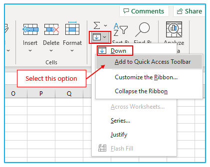
Step 1: Go to the “Fill Down” choice, right-click on it, and select “Add to the Quick Access Toolbar” from the menu that appears.
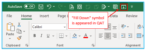
The “Fill Down” symbol should now be visible in the QAT.
4. Using Keyboard Shortcut
You can also use the keyboard shortcut listed below to get the fill-down feature if you prefer that method:
CTRL + D (press the D letter while maintaining the control key)
The methods to fill down the formula using the keyboard shortcut are as follows:
Step 1: Enter the following formula in cell E2:
=D2-C2

Step 2: To implement the formula, select each and every cell (including cell E2).
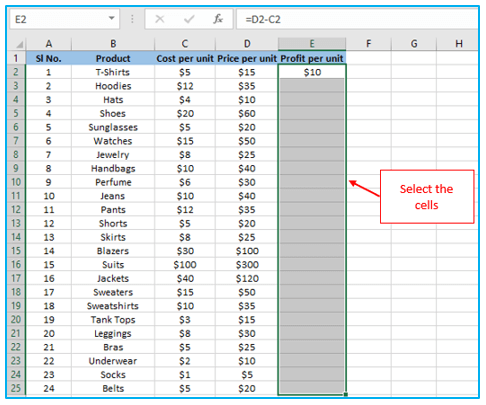
Step 3: Press the D letter while holding down the Control key.

5. Using Array Formula
To apply a formula to the entire column, you can also use the array formula technique if you’re using Microsoft 365 and have access to dynamic arrays.
Let’s say you want to determine the profit in column E using the data set as shown below.
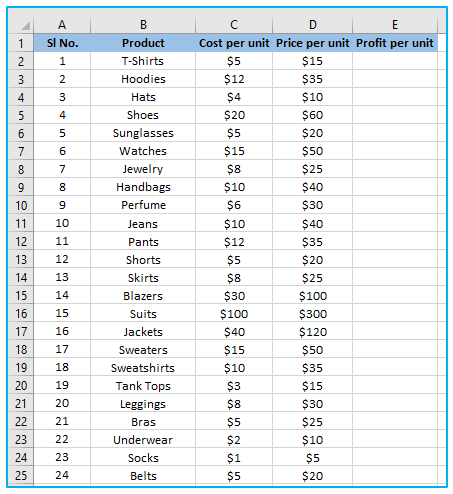
Enter the following formula in cell E2 and see the outcome as shown below.
=D2:D25-C2:C25
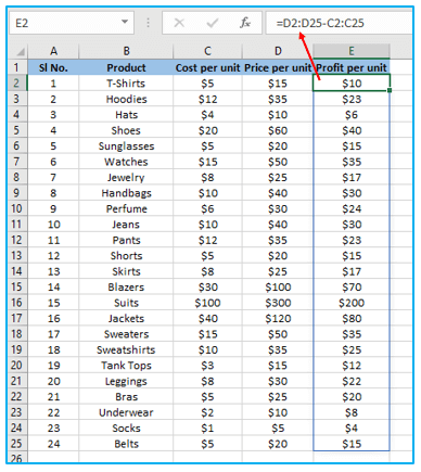
With this array formula, the cell would receive 24 values (one each for E2:E25). However, because we are using dynamic arrays, the outcome would not be limited to a single cell but would instead overflow and fill the full column.
Note: Be aware that not every situation can be solved with this method. In this instance, our formula functions as expected because it takes the input value from an adjacent column and is the same length as the column in which we want the result (i.e., 24 cells).
However, if that’s not the case, then perhaps this isn’t the best method for copying a formula to the complete column.
6. By Copy-Pasting the Cell
Another fast and common way to apply a formula to the whole column (or specific cells within the whole column) is to simply copy the formula-containing cell and paste it over the cells you need it in the column.
Procedure of applying excel formula in entire column is shown below:
Step 1: Enter the following formula in cell E2:
=D2-C2
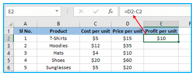
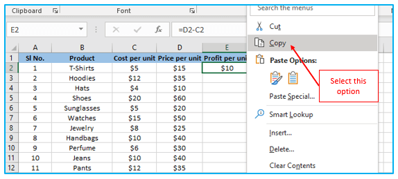
Step 2: Copy the cell (use the keyboard shortcut Ctrl + C in Windows or Cmd + C in Mac).
Step 3: Select each cell where the same formula should be applied (excluding cell E2).
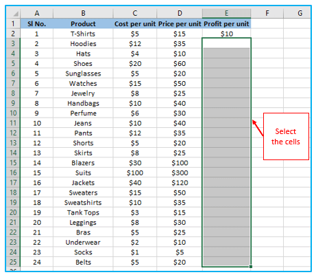
Step 4: Paste the copied cell (Ctrl + V in Windows and Cmd + V in Mac). See the outcome as shown below:

This copy-paste technique differs from all the conversion techniques above it in that you can select to only paste the formula using it (and not paste any of the formatting).
For instance, if cell E2 contains a yellow cell color, all of the methods discussed so far (aside from the array formula method) would paste the formatting (such as the cell color, font size, bold/italics) along with the formula to the complete column
Use the following steps if you only want to implement the formula and not the formatting:
Step 1: Enter the following formula in cell E2:
=D2-C2
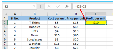
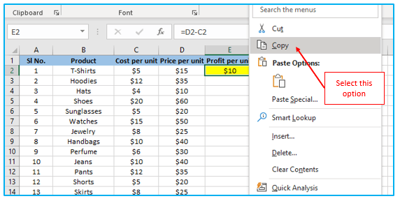
Step 2: Copy the cell (use the keyboard shortcut Ctrl + C in Windows or Cmd + C in Mac).
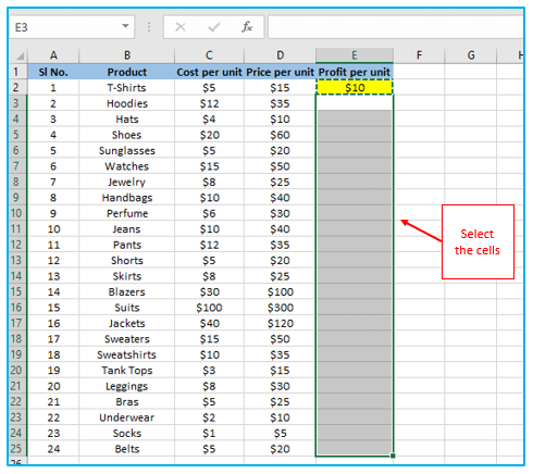
Step 3: Select each cell where the same formula should be applied (excluding cell E2)
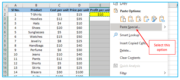
Step 4: Right-click on the selection. Click “Paste Special…” under the list of choices that appears.
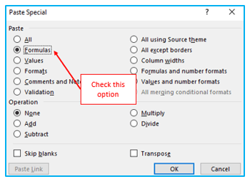
Step 5: Select “Formulas” from the drop-down menu in the “Paste Special” dialog window. Select OK.
The aforementioned actions would guarantee that only the formula was transferred to the chosen cells (and none of the formatting comes over with it).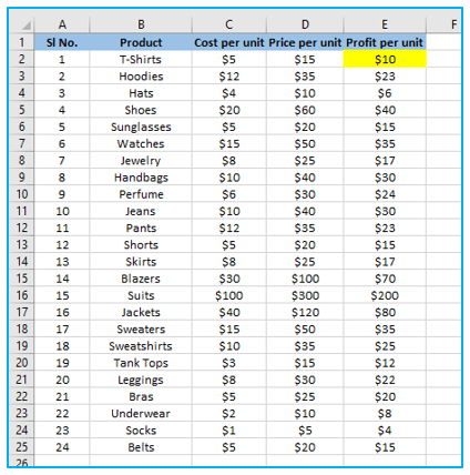
These are some quick and simple techniques for applying a formula to a complete column in Excel.
Application of Apply Formula to Entire Column
- Automated Calculations Across Data Sets:
- Quickly perform calculations like additions, subtractions, or complex formulas across an entire data set, ensuring consistency and saving time compared to manual entry.
- Dynamic Data Analysis:
- Use formulas that automatically adjust when new data is added to a column, ensuring that calculations remain up-to-date and accurate as your data evolves.
- Efficient Data Transformation:
- Apply functions to transform data throughout a column, such as changing text case, formatting dates, or converting units, maintaining uniformity and preparation for analysis.
- Creating Calculated Columns in Tables:
- Add calculated columns in Excel tables to perform dynamic calculations that automatically expand with the table, providing a robust way to manage and analyze related data.
- Conditional Formatting and Data Validation:
- Apply formulas to entire columns to set up conditional formatting rules or data validation criteria, highlighting important information or ensuring data integrity.
- Summarizing and Aggregating Data:
- Use formulas in entire columns to perform summary operations like counting occurrences, averaging values, or finding minimum or maximum values, facilitating quick insights into large data sets.
Applying formulas to entire columns in Excel enhances data processing efficiency, ensures calculation consistency, and opens up a myriad of possibilities for dynamic data analysis and management.
For ready-to-use Dashboard Templates:
