Conditional Formatting Based on Cell Value in Excel transforms your data visualization, allowing for immediate identification of trends, issues, and opportunities within your datasets. By implementing this dynamic tool, you can enhance data analysis, improve readability, and make informed decisions faster. Whether it’s highlighting outliers, tracking progress, or visualizing data distributions, conditional formatting offers a powerful, intuitive way to present and interpret data. Embrace this feature to elevate your Excel skills and bring clarity and efficiency to your reports and analysis.
First, we see how to Apply Conditional Formatting Based on Another Value:
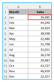
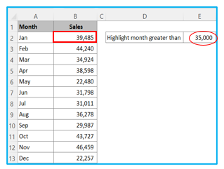
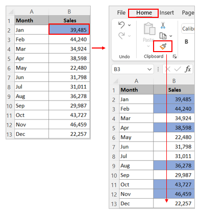
Step 1: From Data set – Select the cell B2
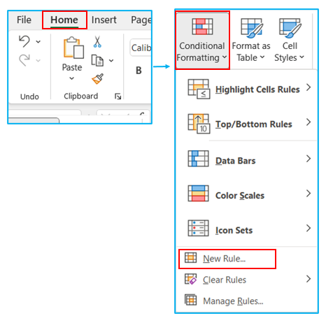
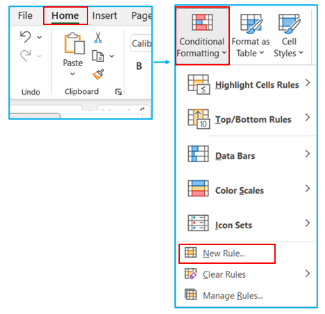
Step 2: Navigate to Home. In the Style area of the ribbon, select the Conditional Formatting.
Step 3: Tap on Conditional Formatting, select ‘New Rule’.
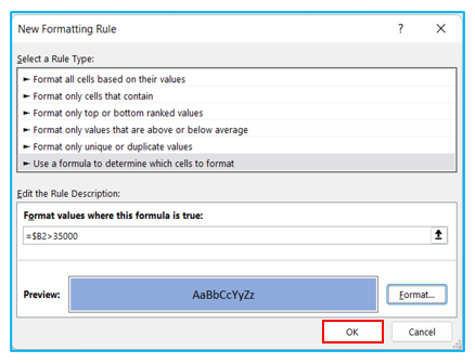
Highlight values more than 35,000
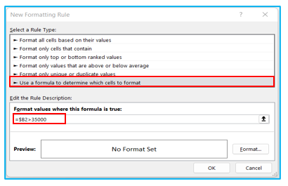
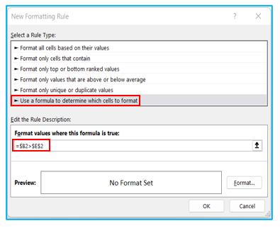
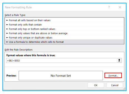
Step 4: Select the “Use a formula to determine which cells to format” option in the New Formatting Rule dialog box.
Step 5: Highlight values more than 35,000. So, Enter the following formula in the field: =$B2>35000.
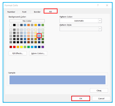
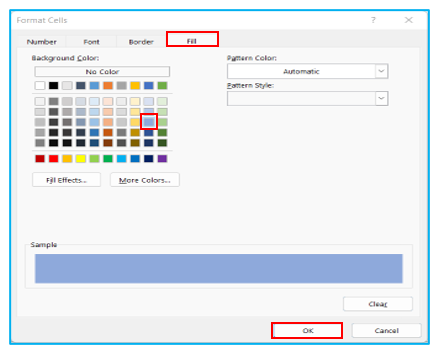
Step 6: Select the Format option (to define how you want the names highlighted).
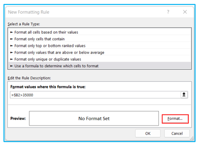
Step 7: Choose the formatting. Then Click OK.
Result Outlined Below. Apply the ‘Format Painter’ from cell B2 to B13.

Now we see how apply Conditional Formatting Based on Another Cell Value
We highlight month value higher than 35,000, i.e., value in cell E2
Step 1: Select the cell to which you like to apply conditional formatting. Here select B2.
Step 2: Navigate to Home. In the Style area of the ribbon, select the Conditional Formatting.
Step 3: Tap on Conditional Formatting, select ‘New Rule’.
Step 4: Highlight values greater than cell value of E2 i.e., 35,000. So, Enter the following formula in the field: =$B2>$E$2.
Step 6: Select the Format option (to define how you want the names highlighted).
Step 7: Choose the formatting. Then Click OK.
Result Outlined Below. Brush the Format Painter from Cell B2 to B13.
Conditional Formatting Based on Cell Value in Excel
Application of Conditional Formatting Based on Cell Value in Excel
You may be interested:
