Pareto Chart in Excel is an invaluable tool for identifying the most significant factors in your data sets, helping you focus on the issues that matter most. By visualizing the 80/20 rule, Pareto Chart in Excel allows you to pinpoint the key contributors to a problem or success, making your analysis more efficient and impactful. Say goodbye to guesswork and hello to data-driven decision-making with this powerful feature. Whether you’re analyzing sales performance, quality control issues, or customer complaints, Pareto Chart in Excel simplifies your data analysis process and drives actionable insights. Take control of your data visualization and improve your analytical outcomes by leveraging the capabilities of Pareto Chart in Excel. With just a few clicks, you can create compelling charts that highlight the vital few from the trivial many, enhancing your ability to prioritize and strategize effectively. Embrace the precision and clarity of Pareto Chart in Excel and elevate your data analysis to new heights of effectiveness and clarity.
This Tutorial Covers:
- What is Pareto chart
- Making a Pareto chart in Excel
- How to make a basic (static) Pareto chart in Excel
- Making a Dynamic (Interactive) Pareto chart in Excel
1. What is Pareto chart?
A Pareto chart combines a line chart and a bar chart, with the line chart serving as a representation of the accumulated total. They are typically used to identify the flaws that should be prioritized in order to see the biggest overall progress. The Pareto principle, called after renowned Italian economist Vilfredo Pareto, serves as the inspiration for the chart.
2. Making a Pareto chart in Excel:
It’s very simple to make a Pareto chart in Excel.
How you organize the data in the backend is where all the trickery is concealed.
In this guide, I’ll demonstrate how to create a:
- Simple (Static) Pareto Chart in Excel.
- Dynamic (Interactive) Pareto Chart in Excel.
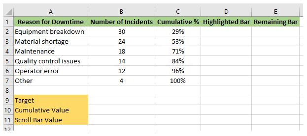
Let’s say you work for a manufacturing company and you want to analyze the reasons for downtime in your production line. You collect data on the causes of downtime over the past month and create the following table:
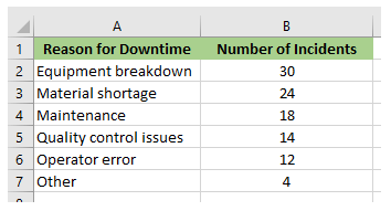
NOTE: You must organize the data in descending order in order to create a Pareto chart in Excel.
-
How to make a basic (static) Pareto chart in Excel?
Static Pareto Chart: There is no choice for the user to view data that correspond to specific values in a static Pareto Chart, which is a basic chart that displays all the data.
The procedures for making a static Pareto chart are as follows:
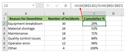
Step 1: Add a new column to C with the name Cumulative Percentage. Next, choose the first box under this column, paste the following formula there, and then use it in all corresponding cells.
Step 2: In the “Charts” section of the “Insert” tab, click the “Insert Column or Bar Chart” drop-down menu after selecting the entire data set (A1:C7). Then select “Clustered Column” from the “2-D Column” option. This adds a column chart with two data sets. (Number of Incidents and the cumulative percentage).
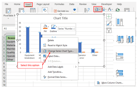
Step 3: Right-click on any of the bars of the Pareto Chart and select “Change Series Chart Type”.
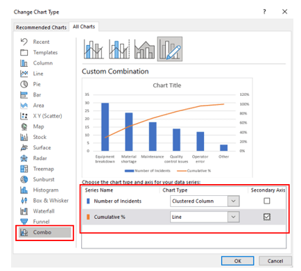
Step 4: In the left pane of the “Change Chart Type” dialogue box, choose “Combo”.
Make the adjustments listed below:
- Number of Incidents: Clustered Column.
- Compound %: Line (also check the “Secondary Axis” check box).
Note: It will be a two-step procedure if you are using Excel 2010 or 2007. First, switch to a line chart as the chart type. After that, right-click the line chart and choose Format Data Series, Secondary Axis, from the Series Options menu.
Your Excel Pareto Chart is prepared. Modify the chart title and vertical axis values.
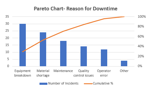
Excel Pareto Chart Interpretation:
This Pareto chart identifies the key problems that the motel should concentrate on in order to resolve the greatest number of complaints. For instance, focusing on the first three problems would resolve 80% of the concerns on their own.
For instance, focusing on the first three problems would resolve 80% of the concerns on their own.
-
Making a Dynamic (Interactive) Pareto chart in Excel:
Dynamic Pareto Chart: A Dynamic Pareto chart is a type of Pareto chart that updates automatically as new data is added or changed. A dynamic Pareto chart is useful when you want to track changes in the data over time, or when the data is updated frequently. With a dynamic chart, you don’t need to manually adjust the chart each time the data changes – the chart will update automatically.
To create a dynamic Pareto chart in Excel, you can use the following steps:
Step 1: Alongside your current data, add the following new columns and rows.
Step 2: Click the “Insert” drop-down menu under the “Controls” portion of the “Developer” tab. Select “Scroll Bar” from the “Form Controls” menu.
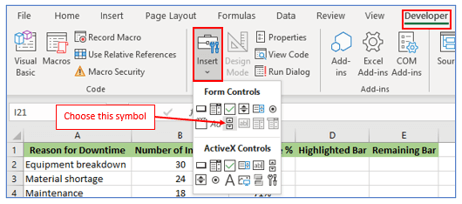
Step 3: Click anywhere on your spreadsheet after selecting “Scroll Bar” from the “Form Controls” menu. The scroll bar looks like below:
Step 4: Resize it to create a horizontal scroll bar that resembles this:
![]()
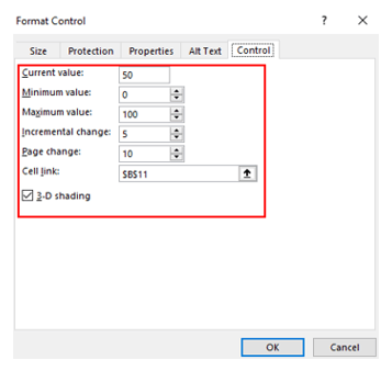
Step 5: Select “Format Control” by performing a right-click on this scroll bar.
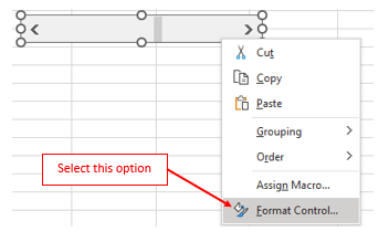
Step 6: In “Format Object” dialog box, adjust your control of the scroll bar. And link the cell B11.
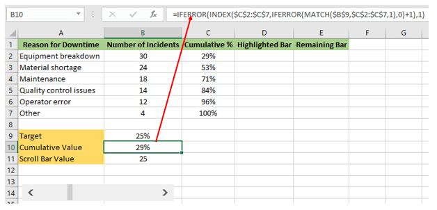
Step 7: Go to cell B9 and enter the formula =B11/100 there. Then, select the B10 cell and enter the following formula:
=IFERROR(INDEX($C$2:$C$7,IFERROR(MATCH($B$9,$C$2:$C$7,1),0)+1),1)
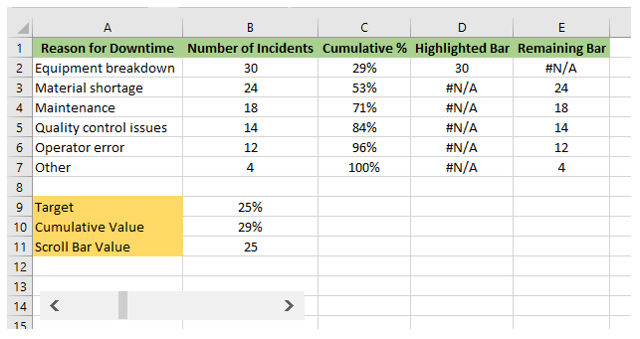
Step 8: Enter the following formula in cell D2 and make sure to apply it to the rest cells of column D.
=IF($B$10>=C2,B2,NA())
Similarly, for cell E2,
=IF($B$10<C2,B2,NA())
The final outcome will be as follows:
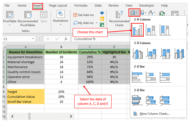
Step 9: In the “Charts” section of the “Insert” tab, click the “Insert Column or Bar Chart” drop-down menu after selecting the entire data from Column A, C, D, and E. Then select “Clustered
Column” from the “2-D Column” option.
Step 10: Select “Change Series Chart” Type by performing a right-click on any of the bars.
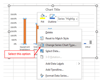
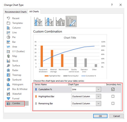
Step 11: Select “Combo” in the left pane of the “Change Chart Type” dialogue panel and make the following adjustments:
- Cumulative %: Line (also check the Secondary Axis checkbox).
- Highlighted Bars: Clustered Column.
- Remaining Bars: Clustered Column.
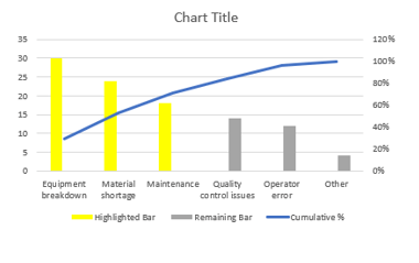
Step 12: To alter the color to Yellow, right-click on any of the highlighted bars.
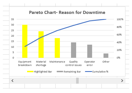
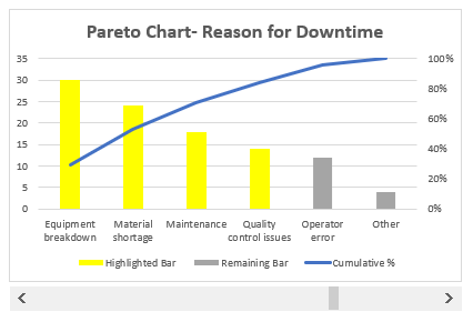
Step 13: Now, place the scroll bar under the Pareto chart and resize it to match the size of the Pareto chart. Name the Pareto chart. You can also modify your vertical axis values.
That concludes the matter!
In Excel, you have produced a dynamic Pareto chart.
The Pareto chart will now update when you adjust the target using the scroll bar.
You can compare the screenshots above and below:
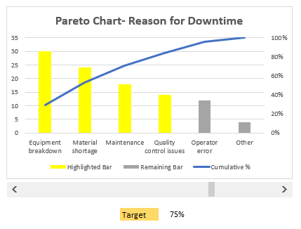
You can do more attractive and understandable the Pareto chart by removing the gridlines and adding the Target value under the scroll bar.
The final Excel dynamic Pareto chart looks like below:
Application of Pareto Chart in Excel
- Identifying Key Issues: Use Pareto Chart in Excel to highlight the most significant problems or defects in a process, allowing you to focus on the areas that will have the greatest impact.
- Sales Analysis: Analyze sales data to determine which products or customers contribute the most to revenue, helping to prioritize marketing efforts and resource allocation.
- Quality Control: Identify the most common sources of defects or errors in manufacturing or service processes, enabling targeted improvements and quality enhancements.
- Customer Complaints: Track and categorize customer complaints to identify the most frequent issues, guiding efforts to improve customer satisfaction and retention.
- Resource Allocation: Determine the most impactful areas for resource allocation by visualizing which factors contribute the most to overall outcomes, optimizing efficiency and effectiveness.
- Process Improvement: Use Pareto Chart in Excel to analyze various steps in a workflow or process, identifying the steps that cause the most delays or inefficiencies for targeted improvements.
For ready-to-use Dashboard Templates:
