The use of Aggregate functions in Excel enables efficient data analysis and summation. They allow users to perform calculations on data sets, extracting valuable information without resorting to manual calculations. Aggregate functions enable users to analyze and summarize data in Excel effectively, facilitating informed decision-making and a deeper understanding of data sets of varying complexity together.
- What is the aggregate function in Excel?
- AGGREGATE Function syntax.
- The Characteristics of the AGGREGATE Function.
- When to use the aggregate function in Excel?
- How to use the aggregate function in Excel? Example-1
- How to use the aggregate function in Excel? Example-2
- How to use the aggregate function in Excel? Example-3
- Some things you need to remember about the Aggregate function.
1. What is the aggregate function in Excel?
The term aggregate function in Excel is used to describe a function that performs calculations on nested data and produces unified output. Excel spreadsheets often require data analysis and summaries that are frequently provided by these functions. By using aggregate functions, users can perform tasks such as adding, averaging, counting (one-to-one), and finding the largest or smallest value rather than using calculations by hand. Excel’s aggregate functions include SUM, AVERAGE, MAX, MIN, COUNT, CoUNTA, COVERTY, SUBFORT, ADAVIFS, and AQUAG.SADDR is an example of this functionality. The functions are designed to enable users to extract valuable insights from their data rapidly and efficiently.
In Excel, aggregate functions are essential tools for analyzing and reporting data, as they help users streamline their workflow and make informed decisions based on Sheets information.
An aggregate function is a formula that you can use in Excel to perform calculations at the same time, and avoid possible errors.
2. AGGREGATE Function syntax.
Aggregate functions in Excel typically follow a particular syntax: =AGGREGATE(function_num, options, ref1, [ref2], …)
Each element is broken down in this manner:
function_num: This is the numeric code that represents the specific aggregate function you want to use. It ranges from 1-19.
For example:
| function_num | Function |
| 1 | AVERAGE |
| 2 | COUNT |
| 3 | COUNTA |
| 4 | MAX |
| 5 | MIN |
| 6 | PRODUCT |
| 7 | STDEV.S |
| 8 | STDEV.P |
| 9 | SUM |
| 10 | VAR.S |
| 11 | VAR.P |
| 12 | MEDIAN |
| 13 | MODE.SNGL |
| 14 | LARGE |
| 15 | SMALL |
| 16 | PERCENTILE.INC |
| 17 | QUARTILE.INC |
| 18 | PERCENTILE.EXC |
| 19 | QUARTILE.EXC |
options: The function can be modified to provide a range of options, including the ability to ignore hidden lines or error values. The value is an integer and can vary depending on the function implemented.
ref1, [ref2]: Those are the numerical values that will be used to perform calculations. At least two of these arguments are required and the remaining arguments are optional. Optional arguments are indicated by square brackets []. Unless you specify an indication or standard, they can be ignored. Even so, including an optional argument implies that all other optional arguments are likewise required.
The array syntax of the AGGREGATE formula is:”=AGGREGATE(function_num),options,array,[k])”
- Array: This is an array of values on which we want to operate
- k: When using functions like LARGE, SMALL, and PERCENTILE.EXC, the operator k is an optional parameter.
3. The Characteristics of the AGGREGATE Function.
The functionality of the AGGREGATE function is as follows:
- function_num values greater than 19 and less than 1 are not recognized.
- For option numbers, the AGGREGATE function does not distinguish between values greater than 7 and less than 1.
- If you enter any other value, you get a “#VALUE! error. “
- Always accepts a number and always returns a number as output.
- Only hidden rows are ignored, but hidden columns are not ignored.
4. When to use the aggregate function in Excel?
When you need to calculate aggregate values more easily, the AGGREGATE function in Excel provides a much more extensive range of options than the standard functions SUM, AVERAGE and MAX.
Using the AGGREGATE function, here are some examples of possible scenarios:
- During the process of data analysis.
When analyzing a set of data, an aggregate function in Excel can be advantageous. While you may have access to company accounting numbers or test results, the aggregate function can be useful for determining trends and creating an equation. In cases where the formatting of a data table is flawed or certain values are not present, this feature can be particularly beneficial.
- when you’re supposed to skip blank rows.
When dealing with a data table that contains numerous empty rows, an aggregate function can be beneficial. By ignoring empty spaces, the function can be executed without an error message while running your calculation. In situations where rearranging a data table is not feasible, aggregate functions can be an effective method to perform calculations.
- To determine the extent of your data.
The use of an aggregate function is beneficial when dealing with a broad data set that requires the knowledge of the maximum and minimum. By using the LARGE function, your formula can determine the largest number that is currently present in the data table. In contrast, the SMALL function can provide the smallest value. By utilizing these functions collectively, you can quickly ascertain the value within your data table.
- During the process of searching your data table for an average.
When searching for the average of data values, consider an aggregate function. The AVERAGE function, which is a subset of the aggregate function can be used to determine the average value. By adding up all the values you input, this equation can calculate the average.
- Performing more complex calculations: Besides addition and averaging, AGGREGATE offers several other functionalities. It is possible to determine percentiles, quartile and median values or perform ranking calculations with AGGREGATE as an example. Statistical analysis and data manipulation can be carried out using this versatile tool.
In essence, the AGGREGATE function in Excel provides more control over aggregate calculations and enables users to handle data analysis and reporting tasks with ease.
5. How to use the aggregate function in Excel? Example-1
To use aggregate the function in Excel as a worksheet function, follow these steps:
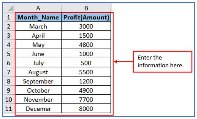
Step 1: The following table contains Every month’s profit of (2022). Make a table with the following data.
Entered the name into the Excel sheet.
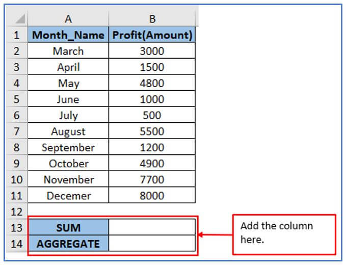
Step 2: Now, add the columns in A13:A14 and B13:B14 to get the SUM and AGGREGATE value.
The column has been added here.
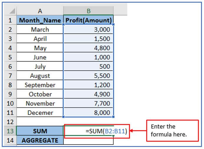
Step 3: Now, run the SUM formula here first. The formula will be: =SUM(B2:B11)
Used the formula here.
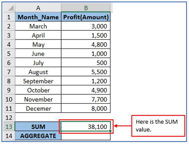
Step 4: After pressing enter you will get the SUM value. Due to the absence of hidden rows, errors, and nested subtotals, the column provides an accurate value.
Here is the Value.
Step 5: Here SUM will be calculated using the AGGREGATE function. The formula of AGGREGATE function will be: =AGGREGATE(9,4,B2:B11)
Applied the formula here.
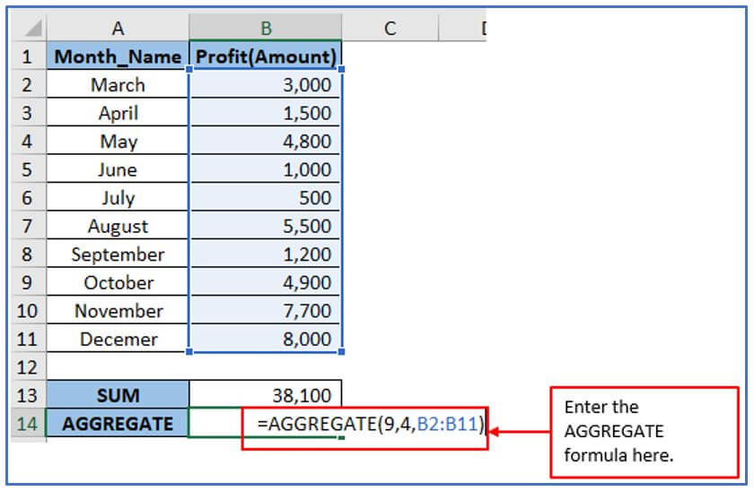
Step 6: Here you can see the result after clicking enter. All values for the Profit of every month are presented, and there is no hiding behind or avoiding any hidden row errors or subtotals (for this we used 4 in the formula for ignoring nothing) that is why the AGGREGATE function also contains the same value as like SUM.
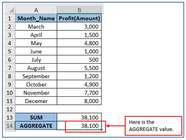
6. How to use the aggregate function in Excel? Example-2
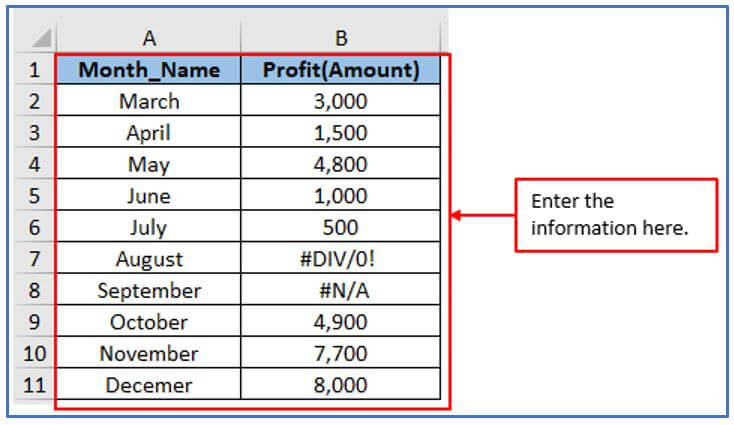
Step 1: First, make some data and put it into Excel as shown in the example. Here taken monthly profit of Data 2022.
All the data has been placed here.
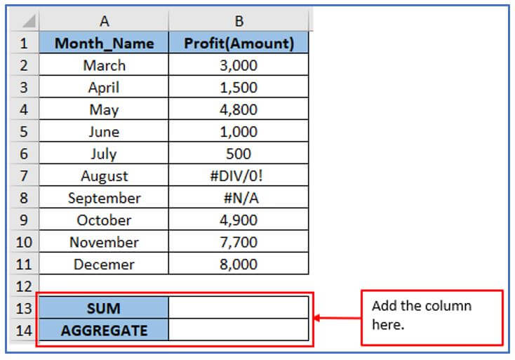
Step 2: You need to add the columns in A13:A14 and B13:B14 to get the SUM and AGGREGATE values.
Added the columns here.
Step 3: Insert the SUM formula. Formula is: =SUM(B2:B11)
Apply the formula in the below image.
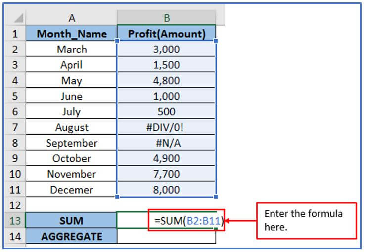
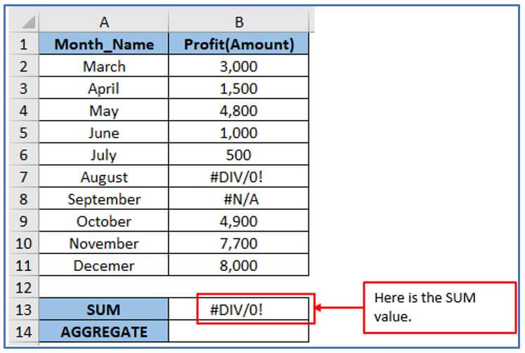
Step 4: Now, press Enter. In column B, there are error values in cells B7 and B8 within the range B2:B11 are referred to as #DIV/0! & #N/A. Due to an error occurring in this range, the error value is returned. Because this column contains #DIV/0! & #N/A.
Here is the result.
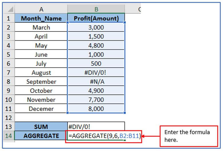
Step 5: In the AGGREGATE formula, when using the appropriate option, AGGREGATE in Excel will give the correct SUM value, ignoring error values. In the AGGREGATE function, we can use option 6 to disregard error values. The AGGREGATE formula: =AGGREGATE(9,6,B2:B11)
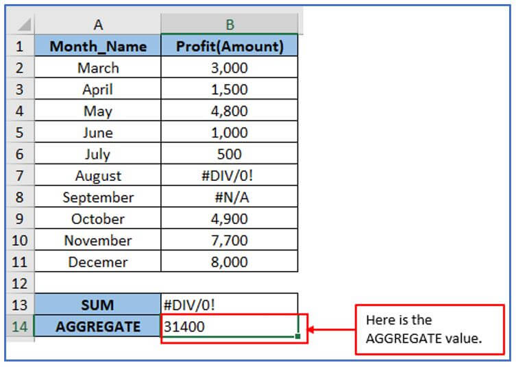
Step 6: The AGGREGATE formula gives the accurate value.
Here is the answer after applying the formula.
7. How to use the aggregate function in Excel? Example-3
Step 1: Make a data table first. Here taken monthly profit of Data 2022.
Place the information here.
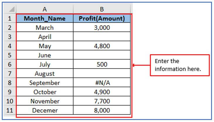
Step 2: Add the columns in A13:A14 and B13:B14 to get the SUM and AGGREGATE values.
Add the columns here.
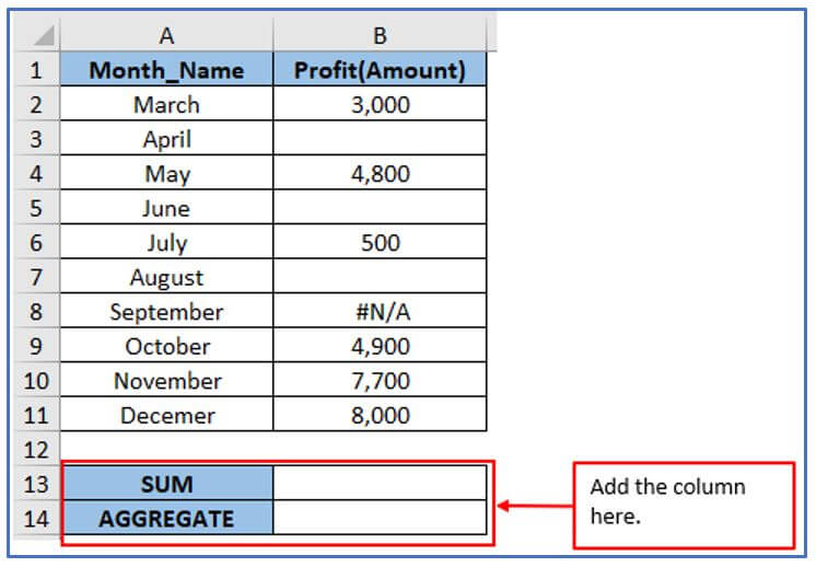
Step 3: Now, Use the SUM formula. The formula: =SUM(B2:B11)
The formula is entered.
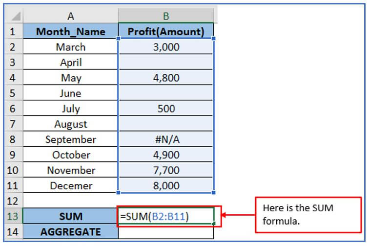
Step 4: After applying the formula click on enter. The error value (#N/A) is found in cell B8, while the range B2:B11 contains a blank cell or hidden row. Due to an error within the given range, the function returns a #N/A error value. The reason is a hidden row or blank value and causing the #N/A error to appear in this column.
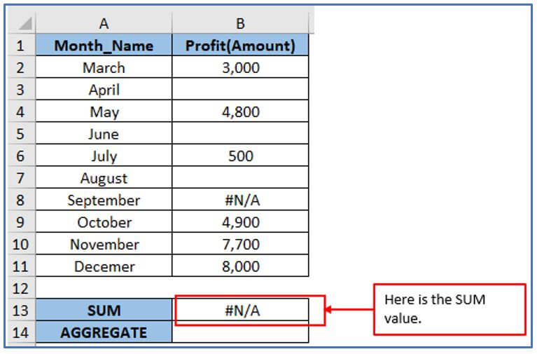
Step 5: Using the correct alternative option in Excel, the AGGREGATE formula will produce the accurate SUM value, disregarding hidden rows and error values. Here using 7 ignore the errors and blank rows.
The formula: =AGGREGATE(9,7,B2:B11)
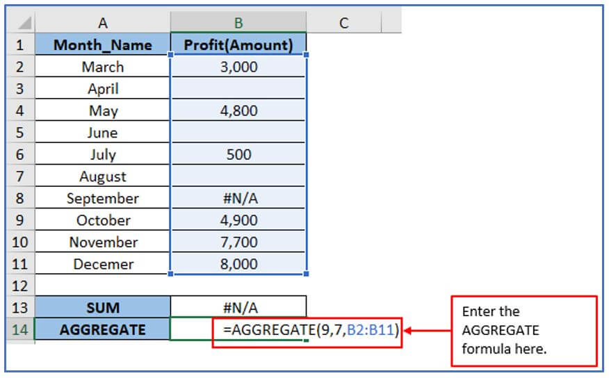
Step 6: After applying the formula click on enter.
Here is the result below.
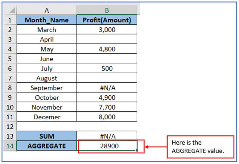
8. Some things you need to remember about the Aggregate function.
- Only vertical ranges or columns of data can be processed by the AGGREGATE function. It does not support horizontal scaling or data flow.
- Hidden columns are not skipped by this function, as it has constraints that only ignore hidden lines.
- The AGGREGATE function applies only to numeric values .
- The value of the _num function argument cannot exceed 19 or be less than 1. The argument must not exceed 7 for options, otherwise, it will provide #VALUE! or error.
- When using the function number range of 14 to 19, which can be LARGE, SMALL, and PERCENTILE.EXC, as arguments for the AGGREGATE function, the operator “K” should be used instead. =AGGREGATE(15, 6, A1: A9, 3) If the k value or the second reference argument is not included, then the value result will be a #VALUE! error.
You may be interested:
