H2: Introduction to Weighted Average in Excel
H3: What is a Weighted Average?
A weighted average is a method used to calculate an average value in which each data point contributes differently to the final result based on its associated weight. Unlike a simple average, where all values are treated equally, a weighted average gives more importance to certain values that carry more significance. For example, in an academic setting, final grades might be calculated by giving exams a higher weight than homework or quizzes. To calculate the weighted average in Excel, you multiply each data point by its corresponding weight, sum these products, and then divide by the total sum of the weights. This approach ensures that the average accurately reflects the significance of each data point within the overall data set. Weighted averages are particularly useful in financial analysis, decision-making processes, and other scenarios where certain data points should have a greater impact on the final average than others.
H3: Why Use a Weighted Average Instead of a Normal Average?
Using a weighted average instead of a normal (simple) average is essential when data points in a data set have varying levels of importance or frequency. In a normal average, each value is treated equally, which might not always provide an accurate representation of the data. For instance, when calculating the average price of products sold, items with higher sales volumes should have more influence on the average than those with fewer sales. By using the weighted average in Excel, you account for these differences by assigning a weight to each data point based on its significance. The SUMPRODUCT function in Excel is a powerful tool that helps you calculate a weighted average efficiently by multiplying each value by its corresponding weight and then dividing the sum of these products by the sum of the weights. This method provides a more accurate reflection of the overall data, making it ideal for complex analyses.
H3: Applications of Weighted Averages in Excel
Weighted averages are widely used across various fields, including finance, education, and economics. In finance, weighted averages are used to calculate the weighted average cost of capital (WACC), which considers the relative proportions of equity and debt in a company’s capital structure. In education, weighted averages help determine final grades by giving different weights to exams, assignments, and quizzes. In inventory management, weighted averages are used to calculate the average cost of goods sold when prices fluctuate over time. Excel is an excellent tool for calculating weighted averages because it offers functions like SUMPRODUCT and SUM that simplify these calculations. By using the SUMPRODUCT function, you can easily multiply each value in a data set by its corresponding weight and then sum the results, providing an accurate and efficient way to analyze data with varying importance.
H2: Understanding the Weighted Average Formula
H3: Basic Weighted Average Formula Explained
The basic weighted average formula in Excel involves multiplying each data point by its corresponding weight, summing these products, and then dividing by the sum of the weights. This can be represented mathematically as:
Weighted Average= ∑(Value×Weight) / ∑Weights
In Excel, this calculation can be performed using the SUMPRODUCT and SUM functions. First, you multiply each value by its corresponding weight using the SUMPRODUCT function. Then, you divide the result by the sum of the weights using the SUM function. This approach ensures that data points with higher weights contribute more to the final average, reflecting their greater importance within the data set. Understanding this formula is crucial for accurately analyzing data where not all values are equally important, such as in financial modeling or academic grading systems. The simple average function is not working here.
H3: How Percentage Weights Affect the Calculation
When calculating a weighted average in Excel, the weights assigned to each data point can be expressed as percentages. These percentage weights indicate the relative importance of each data point within the data set. For example, in a grading system, you might assign 40% weight to the final exam, 30% to midterms, and 30% to homework. To calculate the weighted average using percentage weights, you multiply each data point by its corresponding percentage (expressed as a decimal), sum these products using the SUMPRODUCT function, and then divide by the total sum of the weights, which should add up to 100%. The accuracy of the weighted average calculation depends on correctly applying these percentage weights, as they determine how much each data point influences the final average. Excel’s SUMPRODUCT function is particularly useful for handling percentage weights, making it easier to perform these calculations accurately.
H3: Using the SUM Function to Calculate Weighted Averages
The SUM function in Excel can be used in conjunction with the SUMPRODUCT function to calculate weighted averages. While the SUMPRODUCT function multiplies each value by its corresponding weight and sums the results, the SUM function adds up the total of the weights. To calculate the weighted average, you divide the result of the SUMPRODUCT function by the sum of the weights using the SUM function. For example, if you have a list of grades in column A and their corresponding weights in column B, you would use the formula =SUMPRODUCT(A2:A10, B2:B10) / SUM(B2:B10) to find the weighted average. This method is straightforward and effective for calculating weighted averages in Excel, ensuring that the final average accurately reflects the significance of each data point.
H3: How to Ensure Your Weights Add Up to 100%
When using percentage weights to calculate a weighted average in Excel, it’s important to ensure that the weights add up to 100%. If the weights do not sum to 100%, the final average may not accurately reflect the intended significance of each data point. To check this, you can use the SUM function in Excel to sum the weights. If the sum is not 100%, adjust the weights accordingly to ensure accuracy. For instance, if your weights are in column B, you would use the formula =SUM(B2:B10) to verify the total. Ensuring that the weights add up to 100% is a crucial step in calculating a weighted average, as it guarantees that the final result accurately represents the weighted contribution of each data point in the data set.
H2: Step-by-Step Guide to Calculating Weighted Average in Excel
H3: Setting Up Your Data: Values and Weights
To calculate a weighted average in Excel, you first need to set up your data properly. Start by entering your data points in one column and their corresponding weights in another. For example, you might enter the values in column A and the weights in column B. Ensure that each value is paired with the correct weight, as this pairing will determine how much influence each value has on the final weighted average. Once your data is organized, you can use Excel’s built-in functions to perform the calculation. Setting up your data correctly is the first step toward accurately calculating a weighted average, as it ensures that each data point is weighted appropriately in the final calculation.
H3: Using the SUMPRODUCT Function for Weighted Averages
The SUMPRODUCT function in Excel is a powerful tool for calculating weighted averages. This function multiplies corresponding components in the given arrays and returns the sum of those products. To use the SUMPRODUCT function for a weighted average, you multiply each value in your data set by its corresponding weight and then sum the results. For example, if your values are in column A and weights are in column B, the formula would be =SUMPRODUCT(A2:A10, B2:B10). This formula returns the sum of all the products of the values and their weights, giving you the weighted sum. By dividing this sum by the total sum of the weights, you get the weighted average. The SUMPRODUCT function simplifies the process of calculating weighted averages, making it a preferred method for handling such calculations in Excel.
H3: Excel to Calculate Weighted Average Using SUMPRODUCT
To calculate the weighted average using the SUMPRODUCT function in Excel, follow these steps:
- Enter your data points in one column (e.g., column A).
- Enter the corresponding weights in another column (e.g., column B).
- Use the formula
=SUMPRODUCT(A2:A10, B2:B10) / SUM(B2:B10)to calculate the weighted average.
This formula works by multiplying each data point by its corresponding weight, summing these products, and then dividing by the sum of the weights. The result is the weighted average, which takes into account the relative importance of each data point. This method is particularly useful in scenarios where certain values should have a greater impact on the final average, such as in financial modeling or academic grading. Using the SUMPRODUCT function for weighted averages is a straightforward and efficient way to ensure accurate calculations in Excel.
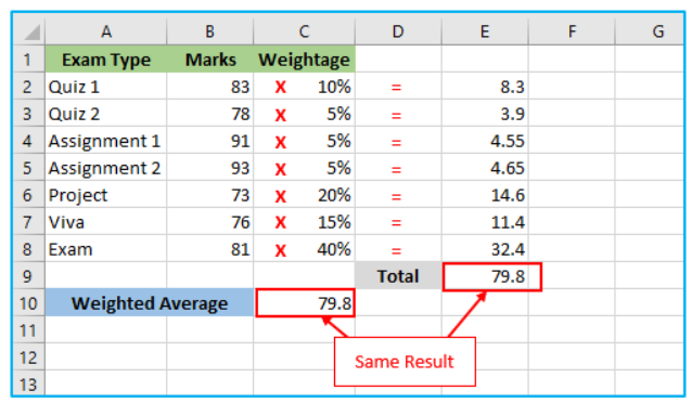
H3: Example Calculation: Weighted Average in a Grading System
Let’s consider an example of calculating a weighted average in a grading system. Suppose a student’s final grade is determined by the following components: homework (30%), midterms (30%), and final exam (40%). The student’s scores are 85 for homework, 90 for midterms, and 95 for the final exam. To calculate the weighted average in Excel:
- Enter the scores in column A (A2).
- Enter the weights (as percentages) in column B (B2).
- Use the formula
=SUMPRODUCT(A2:A4, B2:B4) / SUM(B2:B4)to calculate the weighted average.
This calculation gives you a final grade that accurately reflects the importance of each component. In this example, the formula returns a weighted average score that incorporates the varying significance of homework, midterms, and the final exam. This method ensures that the final grade is a true reflection of the student’s performance, considering the different weights assigned to each component.
H3: Alternative Method: Using the SUM Function for Weighted Averages
While the SUMPRODUCT function is the most efficient way to calculate weighted averages in Microsoft Excel, you can also use the SUM function in combination with other operations. For instance, you can manually multiply each value by its weight, sum these products, and then divide by the sum of the weights. This method is more labor-intensive but can be useful for understanding the underlying mechanics of weighted averages. For example, if you have values in cells A2 to A10 and weights in cells B2 to B10, you could enter the formula =(A2*B2 + A3*B3 + ... + A10*B10) / (B2 + B3 + ... + B10) to calculate the weighted average. This approach provides a more hands-on way to perform the calculation, which can be educational for those learning Excel formulas. However, for large data sets, the SUMPRODUCT function is preferred due to its simplicity and efficiency.
H2: Advanced Tips for Calculating Weighted Averages in Excel
H3: Applying Weighted Averages in Financial Models
Weighted averages are particularly useful in financial models, where different components may contribute unequally to the overall result. For example, in calculating the weighted average cost of capital (WACC), each source of capital, such as debt and equity, is assigned a weight based on its proportion in the company’s capital structure. By using the SUMPRODUCT function in Excel, you can easily calculate these weighted averages, ensuring that your financial models accurately reflect the varying importance of each component. This approach is critical for making informed financial decisions, as it provides a more accurate picture of overall costs and returns. Understanding how to apply weighted averages in financial models is a valuable skill for analysts, accountants, and anyone involved in financial planning or investment analysis.
H3: Using Weighted Moving Averages for Trend Analysis
Weighted moving averages are a powerful tool for trend analysis, particularly in time series data. Unlike simple moving averages, which give equal weight to all data points, weighted moving averages assign more importance to recent data points. This approach makes them more responsive to changes in the data, providing a clearer picture of trends. To calculate a weighted moving average in Excel, you can use the SUMPRODUCT function to multiply each data point by its assigned weight, then divide by the sum of the weights. This method is particularly useful in forecasting and financial analysis, where understanding recent trends is crucial for making predictions. By incorporating weighted moving averages into your analysis, you can gain deeper insights into your data and make more informed decisions.
H3: Common Mistakes to Avoid in Weighted Average Calculations
One common mistake when calculating weighted averages in Excel is failing to ensure that the weights add up to 100%. If the weights do not sum to 100%, the final average may not accurately reflect the intended weighting of the data points. Another mistake is using the wrong formula, such as applying the SUM function without considering the weights, which would result in a simple average instead of a weighted one. Additionally, it’s important to ensure that all data points are correctly paired with their corresponding weights; any mismatches can lead to incorrect calculations. To avoid these errors, double-check your data and formulas before finalizing your calculations. Understanding these common pitfalls can help you avoid inaccuracies and ensure that your weighted averages are calculated correctly.
H3: Excel Tips for Accurate Weighted Average Calculations
For accurate weighted average calculations in Excel, it’s essential to use the right functions and verify your data. The SUMPRODUCT function is the most efficient way to calculate weighted averages, as it automatically multiplies each value by its corresponding weight and sums the results. Additionally, ensure that your weights add up to 100% if you’re using percentage weights, and double-check that each data point is correctly paired with its weight. Using Excel’s error-checking tools can also help identify any issues with your formulas or data. By following these tips, you can ensure that your weighted average calculations are accurate, providing reliable results for your analysis.
H2: Troubleshooting and Optimizing Your Weighted Average Calculations
H3: Handling Missing or Incorrect Weights
When calculating weighted averages in Excel, it’s crucial to handle missing or incorrect weights appropriately. If a weight is missing or set to zero, it can skew the final average, leading to inaccurate results. To avoid this, ensure that every data point has an associated weight and that the weights are correctly entered. If you encounter missing weights, you may need to adjust the existing weights or redistribute them to maintain accuracy. Additionally, using the IFERROR function in Excel can help manage errors that arise from missing weights, ensuring that your calculations remain accurate even when data is incomplete. Properly handling missing or incorrect weights is essential for maintaining the integrity of your weighted average calculations.
H3: How to Adjust Weights Dynamically Using Excel Formulas
In some cases, you may need to adjust weights dynamically based on changing data. Excel allows you to do this using formulas that automatically update weights as the underlying data changes. For example, you can use the SUMIF function to calculate the total weight for specific criteria, and then adjust the weights accordingly. Another approach is to use array formulas that recalculate weights based on the current data set. Dynamic weighting is particularly useful in financial modeling and other applications where data is frequently updated, as it ensures that your weighted averages always reflect the most current information. By leveraging Excel’s powerful formula capabilities, you can create flexible and responsive weighted average calculations.
H3: Verifying Your Results with Excel’s Error Checking Tools
After calculating a weighted average in Excel, it’s important to verify your results to ensure accuracy. Excel offers various error-checking tools that can help identify potential issues with your formulas or data. For instance, the Formula Auditing tools allow you to trace precedents and dependents, making it easier to spot errors in your calculations. Additionally, the IFERROR function can be used to handle potential errors in your weighted average calculations, such as division by zero or missing data. By taking the time to verify your results using these tools, you can ensure that your weighted average calculations are accurate and reliable.
H3: Optimizing Large Data Sets for Weighted Average Calculations
When working with large data sets in Excel, calculating weighted averages can become resource-intensive. To optimize performance, consider using Excel’s array formulas or pivot tables, which can handle large amounts of data more efficiently. Additionally, you can minimize the complexity of your formulas by breaking down the calculation into smaller steps, such as calculating intermediate sums before applying the final weighted average formula. Using named ranges and structured references can also help manage large data sets more effectively, making your formulas easier to read and maintain. By optimizing your approach to calculating weighted averages, you can handle even the largest data sets with ease, ensuring that your analysis is both accurate and efficient.
H2: Conclusion
In this guide, we’ve explored the process of calculating weighted averages in Excel, from setting up your data to applying advanced techniques for dynamic weighting and error checking. We discussed the importance of using weighted averages when data points have different levels of significance, and how to use the SUMPRODUCT function for accurate and efficient calculations. We also covered common mistakes to avoid and tips for optimizing your calculations, particularly when working with large data sets. Understanding these key concepts is essential for anyone looking to perform accurate data analysis in Excel, ensuring that your weighted average calculations reflect the true significance of each data point.
For ready-to-use Dashboard Templates: