How to Display Text in Pivot Table Value Area in Microsoft Excel
Understanding Pivot Table Value Area
A Pivot Table in Microsoft Excel is an essential tool for summarizing and analyzing large datasets. Typically, the Values Area in a Pivot Table is used for numerical calculations, such as sum, average, or count. However, many users want to display text values instead of numbers in this section. By default, text fields are added to the Row Area or Column Area, but not to the Values Area of a Pivot Table. This is because the Values Area is designed to perform calculations.
To work around this, Excel provides several techniques, such as using calculated fields, custom number formats, VBA, and conditional formatting. This guide will walk you through the best methods to display text in Pivot Table Values Area and ensure the desired output without disrupting the table’s core functionality.
Methods to Display Text in the Pivot Table Value Area
Using the PivotTable Field List to Add Text Fields
The PivotTable Field List is an important tool for arranging fields in the Pivot Table. Usually, when you drag the field into the Values Area, Excel automatically applies a numeric function (such as Sum or Count) instead of displaying text. To adjust this:
- Create a Pivot Table by selecting the data and choosing Insert > PivotTable.
- In the PivotTable Field List, select the text field you want to display.
- Drag the text field to the Row Area or Column Area instead of the Values Area to display the text correctly.
- If you want to show text in the Values Area, apply a calculated field or use conditional formatting.
This method ensures that text data appears in the table without defaulting to numerical summarization.
How to Show Text Instead of Numbers in the Values Area
By default, Excel does not allow text values in the Pivot Table Values Area because it is designed to perform calculations. However, you can display text in the Values Area using:
- A Custom Number Format
- Concatenation Techniques
- Data Model Workarounds
To apply a Custom Number Format:
- Right-click the Values Area in the Pivot Table.
- Choose Value Field Settings and click Number Format.
- Select Custom and enter
@in the Type box to force text display.
While this method does not completely replace numbers with text, it helps format text-based results for readability.
Using Conditional Formatting to Display Text
Applying Conditional Formatting for Text Values
Conditional Formatting is a powerful Excel feature that can be used to highlight specific text in a Pivot Table. Since the Values Area typically contains numbers, you can use this method to change how text appears in the table:
- Select the Pivot Table Values Area where you want to display text.
- Click Home > Conditional Formatting > New Rule.
- Choose Use a Formula to Determine Which Cells to Format.
- Enter a formula like: excelCopyEdit
=IF(A2="Yes", "Approved", "Pending") - Set a custom font color or background fill to make text values stand out.
This method does not insert text directly into the Values Area but visually represents conditions based on numerical data.
Formatting Pivot Table Cells Based on Conditions
Since Excel Pivot Tables primarily work with numbers, text-based conditions need to be managed creatively. Here’s how you can format pivot table cells based on conditions:
- Use Conditional Formatting rules to highlight cells containing specific text.
- Convert numbers into text-based labels before inserting them into the Pivot Table.
- Use custom formatting options such as
;;;"TEXT"to replace numbers with pre-defined labels.
This approach is beneficial for tracking statuses, categories, or qualitative data within a Pivot Table.
VBA Method to Display Text in the Pivot Table Value Area
Writing a VBA Script to Show Text in Values
If you need to display text values in the Values Area, VBA (Visual Basic for Applications) is a powerful tool:
- Open Visual Basic Editor (VBE) by pressing
ALT + F11. - Insert a new module and paste the following code: vbaCopyEdit
Sub ConvertTextToPivotValues() Dim pt As PivotTable Dim pf As PivotField Set pt = ActiveSheet.PivotTables(1) For Each pf In pt.DataFields pf.Function = xlMin Next pf End Sub - Run the macro to allow text-based fields in the Values Area.
VBA offers greater flexibility for automating Pivot Table modifications, especially when dealing with text-based values.
Automating Text Display Using Macros
If you frequently need to convert text into Pivot Table Values, creating a macro can save time.
- Macros allow automated formatting, ensuring that text data appears correctly.
- You can define rules for handling non-numeric fields within Pivot Tables.
- Using macros helps maintain consistency in large datasets where text display is necessary.
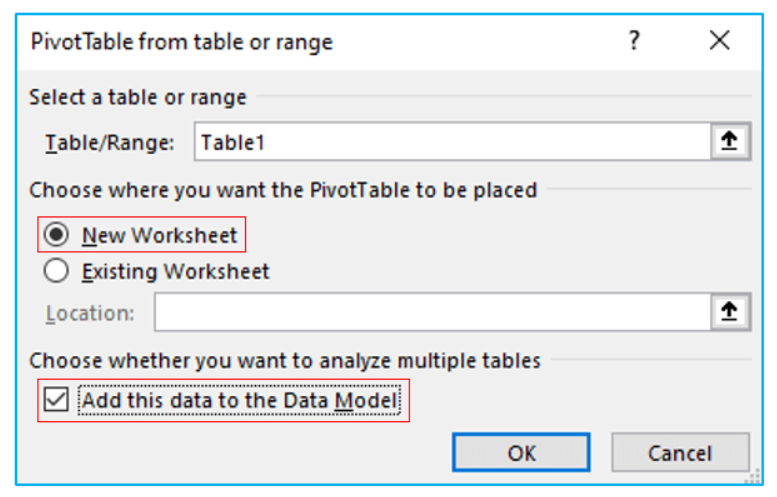
Working with the Data Model for Text Display
Enabling the Data Model for Complex Data
The Data Model in Excel allows users to handle large datasets efficiently. By loading data into the Data Model, you can:
- Use Power Pivot to work with non-numeric values.
- Enable DAX (Data Analysis Expressions) formulas for text handling.
- Avoid default numeric summarization of text-based fields.
This method ensures better data organization while maintaining the integrity of Pivot Table calculations.
Using Power Pivot to Display Text in the Value Area
Power Pivot extends Excel’s capabilities, allowing users to:
- Add text-based calculated fields.
- Modify table relationships to display text categories.
- Create advanced DAX expressions for handling string-based data.
To enable Power Pivot:
- Go to File > Options > Add-ins.
- Select Power Pivot and click Enable.
- Load your data source into Power Pivot and create a new calculated column for text values.
This approach is ideal for businesses handling large datasets with complex text-based reporting needs.
Excel Tips and Tricks for Text in Pivot Tables
Using Calculated Fields to Work Around Limitations
If you want to display text in the Values Area of a Pivot Table, Calculated Fields can help:
- Navigate to PivotTable Analyze > Fields, Items & Sets > Calculated Field.
- Enter a formula that returns a text-based result.
- Apply a custom format to display the text correctly.
This method allows users to override default numeric calculations in Pivot Tables.
Creating a Custom Report with Text Data
Excel Pivot Tables are commonly used for numerical reports, but they can also handle text-based data creatively:
- Use concatenation to merge text fields before adding them to the Pivot Table.
- Format values using Custom Number Formats.
- Create Pivot Charts to visualize text-based data trends.
This ensures that text-based insights are not lost when working with Pivot Tables row and column.
Troubleshooting Issues with Text in Pivot Table Value Area
Common Errors When Displaying Text
Some common issues when working with text fields in Pivot Tables include:
- Text values not appearing in the Values Area.
- Pivot Table defaulting to numeric calculations.
- Formatting issues when displaying text.
To fix these, ensure you use Custom Formats, Calculated Fields, or VBA scripts to manipulate text effectively.
Fixing Issues with PivotTable Field List
If the PivotTable Field List does not show the desired text fields, try:
- Refreshing the Pivot Table (
ALT + F5). - Checking if the data source contains text-based columns.
- Adjusting the Field List settings to enable text display.
By implementing these methods, you can successfully display text in Pivot Table Values Area in Microsoft Excel worksheet.
For ready-to-use Dashboard Templates: